Basics of Light Microscopy Imaging - AOMF

More documents

Recommendations

Info

Box 3: Multiple Image Alignment (mia) Multiple image alignment is a software approach to combine several images into one panorama view having high resolution at the same time. Here, the software takes control of the microscope, camera, motor stage, etc. All parameters are transferred to the imaging system through a remote interface. Using this data, the entire microscope and camera setups can be controlled and calibrated by the software. After defining the required image size and resolution, the user can execute the following steps automatically with a single mouse click: 1. Calculation of the required number of image sections and their relative positions 2. Acquisition of the image sections including stage movement, image acquisition and computing the optimum overlap 3. Seamless “stitching” of the image sections with sub-pixel accuracy by intelligent pattern recognition within the overlap areas. Is there an optimum digital resolution Thus, the number of pixels per optical image area must not be too small. But what exactly is the limit There shouldn’t be any information loss during the conversion from optical to digital. To guarantee this, the digital spatial resolution should be equal or higher than the optical resolution, i.e. the resolving power of the microscope. This requirement is formulated in the Nyquist theorem: The sampling interval (i.e. the number of pixels) must be equal to twice the highest spatial frequency present in the optical image. To say it in different words: To capture the smallest degree of detail, two pixels are collected for each feature. For high resolution images, the Nyquist criterion is extended to 3 pixels per feature. To understand what the Nyquist criterion states, look at the representations in fig. 18 and 19. The most critical feature to reproduce is the ideal periodic pattern of a pair of black and white lines (lower figures). With a sampling interval of two pixels (fig. 18), the digital image (upper figure) might or might not be able to resolve the line pair pattern, depending on the geometric alignment of specimen and camera. Yet a sampling interval with three pixels (fig. 19) resolves the line pair pattern under any given geometric alignment. The digital image (upper figure) is always able to display the line pair structure. With real specimens, 2 pixels per feature should be sufficient to resolve most details. So now, we can answer some of the questions above. Yes, there is an optimum spatial digital resolution of two or three pixels per specimen feature. The resolution should definitely not be smaller than this, otherwise information will be lost. Calculating an example A practical example will illustrate which digital resolution is desirable under which circumstances. The Nyquist criterion is expressed in the following equation: R * M = 2 * pixel size (4) R is the optical resolution of the objective; M is the resulting magnification at the camera sensor. It is calculated by the objective magnification multiplied by the magnification of the camera adapter. Assuming we work with a 10x Plan Apochromat having a numerical aperture (NA) = 0.4. The central wavelength of the illuminating light is l = 550 nm. So the optical resolution of the objective is R = 0.61* l/NA = 0.839 µm. Assuming further that the camera adapter magnification is 1x, so the resulting magnification of objective and camera adaptor is M = 10x. Now, the resolution of the objective has to be multiplied by a factor of 10 to calculate the resolution at the camera: R * M = 0.839 µm * 10 = 8.39 µm. Thus, in this setup, we have a minimum distance of 8.39 µm at which the line pairs can still be resolved. These are 1 / 8.39 = 119 line pairs per millimetre. The pixel size is the size of the CCD chip divided by the number of pixels. A 1/2 inch chip has a size of 6.4 mm * 4.8 mm. So the number of pixels a 1/2 inch chip needs to meet the Nyquist cri- 4. The overlap areas are adjusted automatically for differences in intensity 5. Visualisation of the full view image. 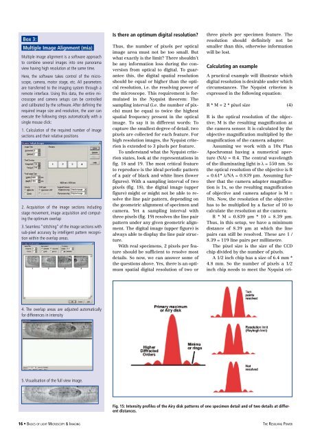Fig. 15: Intensity profiles of the Airy disk patterns of one specimen detail and of two details at different distances. 16 • Basics of light Microscopy & Imaging the Resolving Power
Fig. 16: Airy disk patterns of different size as an example of the resolving power for low NA (left) and high NA (right) objectives. Fig. 17: Four representations of the same image, with different numbers of pixels used. The numbers of pixels is written below each image. terion with 2 pixels per feature, is 1/(R * M) * chip size * 2 = 119 line pairs / mm * 6.4 mm *2 = 1526 pixels in horizontal direction. If you want 3 pixels per line pair, the result is 2289 pixels. This calculation can be followed through for different kind of objectives. Please check out, which numbers of pixels we need for a 1/2 inch chip in table 3. What might be astonishing here is the fact, that the higher the magnification, the fewer pixels the chip of a CCD camera needs! Working with a 100x Plan Apochromat objective combined with an 1/2 inch chip, we need just 800 x 600 pixels to resolve digitally even the finest optically distinguished structure. The higher number of pixels of about 2300 x 1700 is necessary only at lower magnifications up to 10. Which camera to buy The resolution of a CCD camera is clearly one important criterion for its selection. The resolution should be optimally adjusted to your main imaging objective. Optimum resolution depends on the objective and the microscope magnification you usually work with. It should have a minimum number of pixels to not lose any optically achieved resolution as described above. But the number of pixels also should not be much higher, because the number of pixels is directly correlated with the image acquisition time. The gain in resolution is paid for by a slow acquisition process. The fastest frame rates of digital cameras working at high resolution can go up to the 100 milliseconds or even reach the second range, which can become a practical disadvantage in daily work. Furthermore, unnecessary pixels obviously need the same amount of storage capacity as necessary pixels. For example, a 24 bit true colour image consisting of 2289 x 1717 pixels has a file size of almost 12 MB, if there is no compression method applied. The slow frame rate and the file size are just two aspects which demonstrate, that the handling of high resolution images becomes increasingly elaborate. High resolution over a wide field of view The xy-resolution desired is one aspect which makes an image ‘high quality’. Another partially contradicting aspect is that we usually want to see the largest possible fraction of the sample – in best case the whole object under investigation. Here, the microscope’s field of view becomes important. The field of view is given by a number – the so called field number – e.g. if the microscope is equipped for the field number 22 and a 10x magnifying objective is in use, the diagonal of the field of view (via eyepieces and tube that supports the given FN) is 22/10 = 2.2 mm. Using lower magnifying objectives will enable a larger field of view and using large field tubes and oculars can enlarge the field number to 26.5 (e.g. field number 26.5 and 4x objective allows a diagonal of 26.5/4 = 6.624 mm), but unfortunately low magnifying objec- Box 4: Using hardware to increase the resolution in fluorescence microscopy Several hardware components are available, to enable the acquisition of images that are not disturbed by out of focus blur. For example, grid projection, confocal pinhole detection and TIRFM. Since out of focus parts of a specimen produce blur in an image, there is the simple option of eliminating this stray light from the image. With most confocal microscopes, a small pinhole is located in front of the sensor and only those light beams that are originally from the focus area can pass through, others are simply absorbed. The resulting point image only contains information from the focus area. To create an image of more then just one point of the focus area, a scanning process is needed. This scanning process can be performed with the help of spinning disks for an ordinary fluorescence microscope or by a scanning process with a laser beam in a confocal laser scanning microscope (cLSM) set-up. Each system produces different levels of improvement to the resolution. However, all of them need a professional digital sensor system to display the images. TIRFM (Total Internal Reflection Fluorescent Microscopy) uses a completely different concept. With this method, a very thin layer of the specimen (around 200 nm) is used to create the image. Therefore, TIRFM is ideal to analyse e.g. single molecule interactions or membrane processes. To achieve this target, a light beam is directed within a critical angle towards the cover slip. Because of the higher refractive index of the cover slip compared to the specimen, total internal reflection occurs. This means that almost no direct light enters the specimen – but due to the physics of light a so called evanescent wave travels in the specimen direction. This wave is only strong enough to excite fluorochromes within the first few hundred nanometres close to the cover slip. The fluorescent image is restricted to this small depth and cannot be driven into deeper areas of the specimen, and also does not contain out of focus blur from deeper areas. (More information about TIRF can be found at www.olympusmicro.com/primer/techniques/fluorescence/tirf/tirfhome.html). The Resolving Power Basics of light Microscopy & Imaging • 17
Page 1 and 2: Basics of Light Microscopy Imaging
Page 3 and 4: Introduction In this wide-ranging r
Page 5 and 6: “You Can Get Keywords for Expandi
Page 7 and 8: Light How do we describe light that
Page 9 and 10: Fig. 5a-c is showing the emission s
Page 11 and 12: Fig. 6: Schematic of axial chromati
Page 13 and 14: Fig. 11: White balance adjustment u
Page 15 and 16: Human vision For most of us, seeing
Page 17: the resolution which can be reached
Page 21 and 22: quisition. It is called deconvoluti
Page 23 and 24: Box 6: Extended Focal Imaging (efi)
Page 25 and 26: All cats are grey in the dark Why a
Page 27 and 28: Fig. 29: Light path for darkfield c
Page 29 and 30: pixels are grouped in the centre of
Page 31 and 32: (fig. 34). In the condenser, a spec
Page 33 and 34: Where there is light, there is also
Page 35 and 36: Fig. 42: Brightfield image of a dia
Page 37 and 38: A first introduction Most of the ne
Page 39 and 40: act amount needed. The amount of li
Page 41 and 42: Fig. 49: A climate chamber offers f
Page 43 and 44: dyes can be shown as three differen
Page 45 and 46: Reality is multi-dimensional What d
Page 47 and 48: Fig. 57: Left: Height map. Middle a
Page 49 and 50: Fig. 60: Ovariole from Drosophila m
Page 51 and 52: Box 16: The steps involved in 3-D r
Page 53 and 54: Box 18: How is an elemental map of

Basics of Light Microscopy Imaging - AOMF

Create successful ePaper yourself

Delete template?

Save as template?