Basics of Light Microscopy Imaging - AOMF

More documents

Recommendations

Info

Each voxel of a three-dimensional object has a colour. There are several wellknown methods for volume rendering, such as projection and ray casting. These approaches project the three-dimensional object onto the two-dimensional viewing plane. The correct volume generating method guarantees that more than just the outer surface is shown and that the three-dimensional object is not displayed simply as a massive, contourless block. Inner structures within a three-dimensional object, such as fluorescence signals can be visualised. The maximum intensity projection method looks for the brightest voxel along the projection line and displays only this voxel in the two-dimensional view. Fig. 62 shows the maximum intensity projection of two colour channels of 25 frames each when seen from two different angles. Changing the perspective helps to clearly locate the fluorescence signals spatially. The three-dimensional structure will appear more realistic when the structure rendered into three-dimensions is rotated smoothly. How many are there – One or Two Managing several colour channels (each having many z layers) within one image object can be deceptive. The question is whether two structures appearing to overlap are actually located at the same position spatially or whether one is in fact behind the other. The thing is, two fluorescence signals may overlap – because their mutual positions are close to each other within the specimen. This phenomenon is called colocalisation. It is encountered when multi-labelled molecules bind to targets that are found in very close or spatially identical locations. Volume rendering makes it possible to locate colocalised structures in space visually. For better representation and in order to measure colocalisation in digital image objects, the different fluorescence signals are first distinguished from the background. This may be done via Table 4: threshold setting in each of the colour channels. A new image object can be created with only those structures that were highlighted by the thresholds. The colocalised fluorescence signals are displayed in a different colour. Rendering these image objects clearly reveals the colocalised signals without any background disturbance. 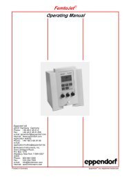To obtain quantitative results, the area fraction of the colocalised signals compared to the total area of each of the two fluorescence signals can be calculated throughout all image sections (see table 4). Layer Red Green Colocalisation Colocalisation/Red Colocalisation/Green Area[%] Area[%] Area[%] Ratio[%] Ratio[%] 1.00 0.11 0.20 0.04 39.60 21.22 2.00 0.15 0.26 0.07 47.76 27.92 3.00 0.20 0.36 0.10 49.93 28.08 4.00 0.26 0.53 0.13 51.84 25.32 5.00 0.35 1.34 0.20 57.39 14.87 6.00 0.43 2.07 0.26 61.00 12.81 7.00 0.38 1.96 0.24 61.66 12.07 Colocalisation sheet: A ratio value of about 52 % in the Colocalisation/Red column in layer 4 means that 52 % of red fluorescence signals are colocalised with green fluorescent structures here. 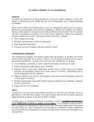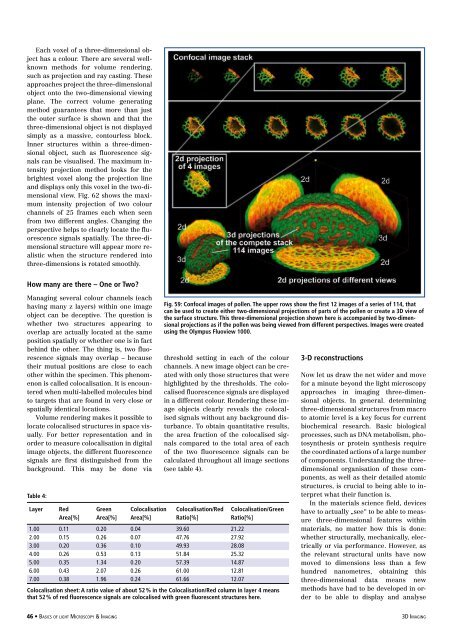Fig. 59: Confocal images of pollen. The upper rows show the first 12 images of a series of 114, that can be used to create either two-dimensional projections of parts of the pollen or create a 3D view of the surface structure. This three-dimensional projection shown here is accompanied by two-dimensional projections as if the pollen was being viewed from different perspectives. Images were created using the Olympus Fluoview 1000. 3-D reconstructions Now let us draw the net wider and move for a minute beyond the light microscopy approaches in imaging three-dimensional objects. In general. determining three-dimensional structures from macro to atomic level is a key focus for current biochemical research. Basic biological processes, such as DNA metabolism, photosynthesis or protein synthesis require the coordinated actions of a large number of components. Understanding the threedimensional organisation of these components, as well as their detailed atomic structures, is crucial to being able to interpret what their function is. In the materials science field, devices have to actually „see“ to be able to measure three-dimensional features within materials, no matter how this is done: whether structurally, mechanically, electrically or via performance. However, as the relevant structural units have now moved to dimensions less than a few hundred nanometres, obtaining this three-dimensional data means new methods have had to be developed in order to be able to display and analyse 46 • Basics of light Microscopy & Imaging 3D Imaging
Fig. 60: Ovariole from Drosophila melanogaster mutant bgcn. Multicolour channel and z stack images can be managed in one image object. This image object contains three colour channels each consisting of a 41 frame z stack. This image is a maximum intensity projection. Red: Fascilin III, Green: F-Actin, Blue: Nuclei. Above right: Single z layer after applying the blind deconvolution algorithm to all three channels of the image object. Left: The three-dimensional, volume-rendered structure. Image courtesy of: Dr. Ralph Rübsam, Institute for Biology, University of Erlangen-Nürnberg, Erlangen, Germany. three-dimensional structures. Among these methods, different 3-D reconstruction approaches have become a useful tool in various applications in both the life and materials sciences. They result in three-dimensional displays which are particularly illustrative and instructive. Therefore, we now take a closer look at two of these 3-D reconstruction methods, one using an image series of specimen sections acquired in a light microscope, the second using electron tomography in a transmission electron microscope. 3-D Reconstruction using an image series of specimen sections One commonly used method when dealing with 3-D reconstruction is to make a series of ultra-thin slices of the specimen being investigated. These slices are then dyed. The dye makes structures more easily recognisable and/or highlights specific parts. The slices are viewed one at a time beneath the microscope and drawn. These drawings are then enlarged to scale. In the past, a 3-D model was reconstructed layer by layer from pieces of cardboard cut according to the drawings. Alternatively, wax or plastic was used to make the model. Today, this is greatly simplified by the computer assembling the virtual model. Special 3-D programmes calculate the three-dimensional model based on digitised image slices. This model is referred to as a 3-D reconstruction. Today‘s powerful software offers 3-D processing, display and evaluation of two-dimensional image information. Ergonomic functions and flexible project management provide the user with the ability to reconstruct even the most complex models, and allow easy access to spatial views of the interiors of such structures. Up until now, these interior views were extremely difficult to generate. Box 16 shows the necessary steps of 3-D reconstruction, such as those used for displaying embryonic growth processes in three dimensions. This approach is attractive for research conducted in other areas as well – such as the materials sciences. 3-D reconstruction by tilting the specimen Tomography is another way of reconstructing the three dimensional (3-D) structure of a specimen from a series of two dimensional (2-D) micrographs. Some sample tomography applications include not only those for electron microscopy (called electron tomography) but also * eucentric is derived from the Latin for well-centered. It implies, e.g., in a goniometer and especially in a specimen stage, that the specimen can be tilted without moving the field of view. This capability is highly desirable for microscope stages. Fig. 61: This is how a two-dimensional pixel (picture element) is expanded to a three-dimensional voxel (volume element). 3D Imaging Basics of light Microscopy & Imaging • 47
Page 1 and 2: Basics of Light Microscopy Imaging
Page 3 and 4: Introduction In this wide-ranging r
Page 5 and 6: “You Can Get Keywords for Expandi
Page 7 and 8: Light How do we describe light that
Page 9 and 10: Fig. 5a-c is showing the emission s
Page 11 and 12: Fig. 6: Schematic of axial chromati
Page 13 and 14: Fig. 11: White balance adjustment u
Page 15 and 16: Human vision For most of us, seeing
Page 17 and 18: the resolution which can be reached
Page 19 and 20: Fig. 16: Airy disk patterns of diff
Page 21 and 22: quisition. It is called deconvoluti
Page 23 and 24: Box 6: Extended Focal Imaging (efi)
Page 25 and 26: All cats are grey in the dark Why a
Page 27 and 28: Fig. 29: Light path for darkfield c
Page 29 and 30: pixels are grouped in the centre of
Page 31 and 32: (fig. 34). In the condenser, a spec
Page 33 and 34: Where there is light, there is also
Page 35 and 36: Fig. 42: Brightfield image of a dia
Page 37 and 38: A first introduction Most of the ne
Page 39 and 40: act amount needed. The amount of li
Page 41 and 42: Fig. 49: A climate chamber offers f
Page 43 and 44: dyes can be shown as three differen
Page 45 and 46: Reality is multi-dimensional What d
Page 47: Fig. 57: Left: Height map. Middle a
Page 51 and 52: Box 16: The steps involved in 3-D r
Page 53 and 54: Box 18: How is an elemental map of

Basics of Light Microscopy Imaging - AOMF

You also want an ePaper? Increase the reach of your titles

Delete template?

Save as template?