10 07 29 Master thesis Juliana Leon - e-Waste. This guide

More documents

Recommendations

Info

Table 7: Average composition and weight of CPU, Laptop, CRT-monitor and LCD-monitor used in this study. Material Level 1 → CPU (1) Laptop (2) CRT-monitor (3) LCD-monitor (4) ↓ Material Level 2 kg/CPU (%) kg/laptop (%) kg/CRT (%) kg/LCD (%) Ferrous metals 6.700 67.00% 0.554 18.47% 1.250 10.42% - - Aluminium 0.380 3.80% 0.168 5.60% 0.200 1.67% 0.550 11.00% Copper 0.120 1.20% 0.014 0.47% 0.500 4.17% 0.010 0.20% Brass 0.020 0.20% - - - - - - Metals (non defined) - - 0.560 18.67% - - - - PWBs 1.320 13.20% 0.410 13.67% 1.200 10.00% 0.220 4.40% Plastics 0.810 8.10% 0.420 14.00% 2.400 20.00% 1.900 38.00% CRT - - - - 6.450 53.75% - - Screen - - 0.600 20.00% - - 2.320 46.40% Batteries, capacitors 0.080 0.80% 0.274 9.13% - - - - Other waste 0.220 2.20% - - - - - - Copper (from wires) 0.220 2.20% - - - - - - Plastic (from wires) 0.130 1.30% - - - - - - Total weight (kg) 10.000 3.000 12.000 5.000 (1) Adapted from Gmünder (2007), Ministerio de Comunicaciones et al. (2008) and Laffely (2007) (2) Adapted from Ecoinvent data v2.01 found in Wolfensberger (2010) (3) Adapted from Marthaler (2008), Laffely (2007) and Ministerio de Comunicaciones et al. (2008) (4) Adapted from Ecoinvent data v2.01 found in Wolfensberger (2010) 2.3.5 Mathematical description Let the number of flows in the system be n, the number of goods be q and the number of materials be p. According to the mass balance principle, the mass of all inputs entering a process equals the mass of all outputs of this process plus a storage term that takes into account accumulation or depletion of materials in the process. This principle is valid for total flows (Equation 5) as well as for individual material flows (Equation 6). ∑ n I F ˙ input = ∑ F ˙ output + F ˙ storage (5) n O € ∑ n I m ˙ input = ∑ m ˙ output + m ˙ storage (6) n O As expressed in Equation 7, the aggregated flow for a material ( M ˙ ) is composed by the sum of material € flows in each good ( m ˙ ). q € M ˙ k ij = ∑ m ˙ ij (7) k =1 € € 16
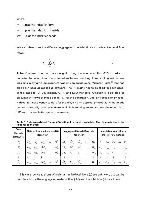
where: i=1,…,n as the index for flows j=1,…,p as the index for materials k=1,…,q as the index for goods We can then sum the different aggregated material flows to obtain the total flow rates. p F ˙ i = ∑ M ˙ ij (8) j =1 Table 8 shows how data is managed during the course of the MFA in order to consider for € each flow the different materials resulting from each good. A tool including a dynamic spreadsheet was implemented using Microsoft Excel ® that has also been used as modelling software. The m ˙ -matrix has to be filled for each good, in this case for CPUs, laptops, CRT- and LCD-monitors. Although it is possible to calculate the flows of these goods ( G ˙ ) for the generation, use, and collection phases, ! it does not make sense to do it for the recycling or disposal phases as entire goods do not physically exist any € more and their forming materials are dispersed in a different manner in the system processes. Table 8: Data spreadsheet for an MFA with n flows and p materials. The filled for each good. ˙ m matrix has to be € € € € € Total flow rate (tons/year) ˙ F 1 ˙ F 2 ˙ € € ˙ € F 3 F n € € € Material flow rate from good G k k m ˙ 11 j m ˙ 21 k m ˙ 12 j m ˙ 22 j m ˙ 31 € € j m ˙ n1 ˙ € j m ˙ 32 (tons/year) € j € € € € m n 2 k m ˙ 13 j m ˙ 23 j ˙ € € j ˙ € m 33 m n 3 € € € k m ˙ 1p j m ˙ 2 p ˙ j m 3 p ˙ € € k m np € Aggregated Material flow rate ˙ M 11 ˙ M 21 ˙ M 31 ˙ M n1 € € € ˙ M 12 ˙ M 22 ˙ M 32 (tons/year) € € € € € ˙ M 13 ˙ M 23 ˙ € € ˙ € M 33 € € € ˙ M 1p ˙ M 2p ˙ € ˙ € € M 3p Material concentration in c 11 c 21 c 31 € € € the total flow (kg/tons) € € € € € € € € € € € € € In this € case, € concentrations € € of materials € € in the total € flows € (c) are € unknown, € but € can be calculated once the aggregated material flow ( M ˙ ) and the total flow ( F ˙ ) are known. ˙ M n 2 M n 3 ! M np c n1 c 12 c 22 c 32 € € € € € c n 2 c 13 c 23 c 33 € € c n 3 € c 1p c 2 p c 3 p c np € 17 €
Page 3 and 4: Abstract In Colombia, as in other d
Page 5 and 6: Glossary Chatarrerías - A term use
Page 7 and 8: 3.3.2 Informal refurbishment and r
Page 9: List of Tables Table 1: General inf
Page 12 and 13: 1.2 Colombia as case study The Repu
Page 14 and 15: (both laptop and desktop) in Colomb
Page 16 and 17: collection, refurbishment, manual d
Page 18 and 19: 2 METHODS 2.1 Computer waste genera
Page 20 and 21: Table 4: Parameters used for the co
Page 22 and 23: made. This means that from the tota
Page 24 and 25: 2.3.1 Definitions The following imp
Page 28 and 29: M c ik = ˙ ik ˙ (9) F i The distr
Page 30 and 31: In 2009, waste of more recent techn
Page 32 and 33: 200 and 350 tons. Based on the latt
Page 34 and 35: iggest formal e-waste recycling com
Page 36 and 37: this study, the term “informal co
Page 38 and 39: A pilot project conducted in Bogot
Page 40 and 41: Figure 12: Manual dismantling of co
Page 42 and 43: city. Scrap metal dealers are then
Page 44 and 45: The direct MSW collection rate is t
Page 46 and 47: In the three scenarios, informally
Page 48 and 49: are mixed with common glass, or are
Page 50 and 51: entering the market are almost excl
Page 52 and 53: Non treated (low-grade PWBs) Formal
Page 54 and 55: Refurbish Formal treatment Worst ca
Page 56 and 57: introduction of an Advanced Recycli
Page 58 and 59: Table 15: Theoretical benefit from
Page 60 and 61: 3.5.1.3 Social benefits Allowing th
Page 62 and 63: 3.5.2.2 Environmental benefits Evid
Page 64 and 65: 4 FINAL REMARKS 4.1 Computer waste
Page 66 and 67: possible intervention points. There
Page 68 and 69: small metal parts that can be sold,
Page 70 and 71: 6 ACKNOWLEDGEMENTS I would like to
Page 72 and 73: Gmünder S. (2007). Recycling - Fro
Page 74 and 75: Uribe L.M., Wolfensberger M. y Ott,
Page 76 and 77:
Appendix A.2: List of expert interv
Page 78 and 79:
Appendix B.1: Flow scheme for the
Page 80 and 81:
Appendix C.2: Flow Matrix for the
show all

10 07 29 Master thesis Juliana Leon - e-Waste. This guide

Create successful ePaper yourself

Delete template?

Save as template?