Wind field simulations at Askervein hill - WindSim
Wind field simulations at Askervein hill - WindSim
Wind field simulations at Askervein hill - WindSim

Create successful ePaper yourself
Turn your PDF publications into a flip-book with our unique Google optimized e-Paper software.
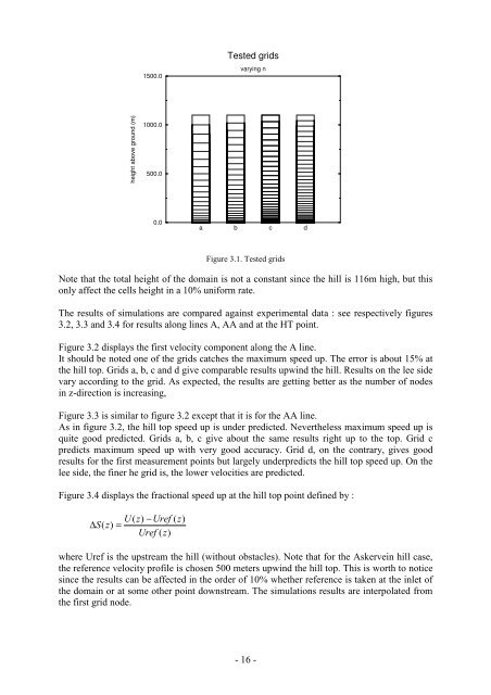
1500.0<br />
Tested grids<br />
varying n<br />
height above ground (m)<br />
1000.0<br />
500.0<br />
0.0<br />
a b c d<br />
Figure 3.1. Tested grids<br />
Note th<strong>at</strong> the total height of the domain is not a constant since the <strong>hill</strong> is 116m high, but this<br />
only affect the cells height in a 10% uniform r<strong>at</strong>e.<br />
The results of <strong>simul<strong>at</strong>ions</strong> are compared against experimental d<strong>at</strong>a : see respectively figures<br />
3.2, 3.3 and 3.4 for results along lines A, AA and <strong>at</strong> the HT point.<br />
Figure 3.2 displays the first velocity component along the A line.<br />
It should be noted one of the grids c<strong>at</strong>ches the maximum speed up. The error is about 15% <strong>at</strong><br />
the <strong>hill</strong> top. Grids a, b, c and d give comparable results upwind the <strong>hill</strong>. Results on the lee side<br />
vary according to the grid. As expected, the results are getting better as the number of nodes<br />
in z-direction is increasing,<br />
Figure 3.3 is similar to figure 3.2 except th<strong>at</strong> it is for the AA line.<br />
As in figure 3.2, the <strong>hill</strong> top speed up is under predicted. Nevertheless maximum speed up is<br />
quite good predicted. Grids a, b, c give about the same results right up to the top. Grid c<br />
predicts maximum speed up with very good accuracy. Grid d, on the contrary, gives good<br />
results for the first measurement points but largely underpredicts the <strong>hill</strong> top speed up. On the<br />
lee side, the finer he grid is, the lower velocities are predicted.<br />
Figure 3.4 displays the fractional speed up <strong>at</strong> the <strong>hill</strong> top point defined by :<br />
U(<br />
z)<br />
−Uref<br />
( z)<br />
∆ S(<br />
z)<br />
=<br />
Uref ( z)<br />
where Uref is the upstream the <strong>hill</strong> (without obstacles). Note th<strong>at</strong> for the <strong>Askervein</strong> <strong>hill</strong> case,<br />
the reference velocity profile is chosen 500 meters upwind the <strong>hill</strong> top. This is worth to notice<br />
since the results can be affected in the order of 10% whether reference is taken <strong>at</strong> the inlet of<br />
the domain or <strong>at</strong> some other point downstream. The <strong>simul<strong>at</strong>ions</strong> results are interpol<strong>at</strong>ed from<br />
the first grid node.<br />
- 16 -