Wind field simulations at Askervein hill - WindSim

ν T
= l m
U
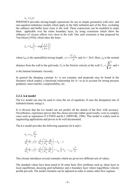
PHOENICS provides mixing-length expressions for use in simple geometries with zero- and
one-equation turbulence models which apply in the fully turbulent part of the flow, excluding
the sublayer and buffer layer close to the wall. These expressions can be modified to make
them applicable over the entire boundary layer, by using extensions which allow the
influence of viscous effects very close to the wall. One such extension is that proposed by
Van Driest [1956], which takes the form:
l
m
= l
m0
⎛ ⎛
⎜1
− exp⎜
⎝ ⎝
y
A
+
+
⎞⎞
⎟⎟
⎠⎠
Uτ
y
g
where l m0 is the unmodified mixing length, y + = and A+= 26.0. Here, y g is the normal
ν
τ
w
distance from the wall to the grid node, U τ is the friction velocity at the wall U
τ
= and ν
ρ
is the laminar kinematic viscosity.
In general the damping constant A+ is not constant, and proposals may be found in the
literature which employ a functional relationship for A+ so as to account for strong pressure
gradients, mass transfer, compressibility, etc.
2.2.2. k-ε model
The k-ε model can also be used to close the set of equations. It uses the dissipation rate of
turbulent kinetic energy ε.
It is obvious that the k-ε model can not predict all the details of the flow with accuracy.
Nevertheless, experience proves that this choice provides rather good results, even in complex
cases such as separation (T.UTNES and K.J. EIDSVIK, 1996). This model is widely used in
engineering applications and proves to be well documented.
The k-ε model provides the following equations for k and ε :
νT c k 2
=
µ
ε
( U k i )
∂
∂ ⎛ ν
T ∂ k ⎞
=
ε
∂ x ∂ x ⎜ σ ∂ x ⎟ + P −
i
i ⎝ k i ⎠ k
∂
∂ ⎛ ν ∂ ε ⎞ ε
∂
( U ε
T
x i ) = ⎜ ⎟ c
∂ x ⎜ σ ∂ x ⎟ + ε k P c
k
− ε
i i ⎝ ε i ⎠
1 2
ε
2
k
This closure introduces several constants which are given two different sets of values.
The standard values have been tuned to fit some basic flow problems such as, shear layer in
local equilibrium, decaying grid turbulence and a boundary layer where logarithmic velocity
profile prevails. The model constants can be adjusted in order to mimic other flow regimes.
- 9 -