UM-0046-A0 - DT500 Concise Users Manual - dataTaker

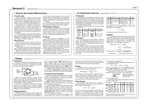
Sensors 2 ... understanding helpsHints for Successful MeasurementGround LoopsGround loops are a common cause of manymeasurement problems, including noise, offsets anderratic behaviour. Ground loops occur when a circularconduction path is established between grounds in asystem. The use of differential inputs instead of singleended inputs overcomes most ground loop problems.Fundamental to the condition is the incorrectassumption that there is a single ground potential in ameasurement system. In practice, two grounds in asystem are rarely at the same potential. The result isthat ground currents are very common, and if allowed toflow through the sensor wiring then measurement errorsare inevitable.The communications cable often creates a groundloop. If disconnecting the COMS cable has an effect onlogged data, this suggests a poor wiring arrangement.Isolating the COMS port normally solves the problem(see "COMS Port Isolation" on page 13).Noise Pick-upThere are two main ways in which noise can beintroduced into signal wiring: by capacitive coupling andby magnetic induction. There are different countermeasures for each.Shielding signal wiring will minimise capacitive noisepick-up. Signal wiring that is close to line voltage cableshould always be shielded (see "Config 1" on page 19).Magnetic induction of noise from current carryingcables or from electrical machines (especially motorsand transformers) is a greater problem. Shielded cableis not an effective counter-measure. The only practicalmeasures are to avoid magnetic fields, and to use closetwisted conductors for the signal wiring. Shielding insteel pipe can be effective, but is generally not economicor convenient.The influence of noise can be minimised using theESn channel option (see "Extra Samples" on page 5)and averaging (see "Statistical Channels" on page 6).Self Heating of SensorsSensors that need excitation power to be read areheated by power dissipation. This can be particularlyacute with temperature sensors and some sensitivebridges. Minimise error by minimising the excitationpower, exciting only when needed (by using the exciteterminal), or by calibrating out steady state errors.AccuracyThe basic accuracy of the Datataker is 0.1% ofreading (not full scale) plus a small offset error (4µV,40µV and 400µV) for each voltage measurement rangeat 25°C. The temperature coefficient for the scale factoris 20ppm/°C max. Any one of the three basic rangesmay be trimmed to 0.003% by trim-pot or P1. TheDatataker self calibrates its measurement circuitswhenever its input voltage offset drifts by more than avalue set by P0 in microvolts (defaults to 4µV).The calibration procedure employs two standards - a2.500V (20ppm/°C) voltage reference and a 100.0Ω(10ppm/°C) reference resistor. You can trim these withP1 and P3 (see "Parameters" on page 11).IC Temperature Sensors ... wiring configs. 18, 19, 20, 21IntroductionIntegrated Circuit (IC) temperature sensors are devicesthat are constructed on small silicon chips. These are linear,sensitive and available in both voltage and current outputconfigurations. They share the thermistor's disadvantage oflimited temperature range (generally –40°C to +150°C) andself-heating from power dissipation caused by the excitationcurrent needed to read the sensor.Datataker supports the four most commonly availableIC sensor types:Sensor Output Channel Type Wiring Config.AD590* 1µA/°K nAD590 18, (7, 8)& AD592*LM34** 10mV/°F nLM34 20, 21, (1, 2, 3)LM35** 10mV/°C nLM35 20, 21, (1, 2, 3)LM335** 10mV/°K nLM335 19, (4, 5, 6)CalibrationIC temperature sensors have different calibrationgrades. The lowest grades typically have an error of up to±2°C at 25°C. More expensive sensors have an error of±0.25°C. This error is a combination of an offset (or zero)error and a slope error.The Datataker provides a slope (or scale) correctioncapability on a per sensor basis using the channel factor.See "Channel Types" on page 4 and "Channel Options" onpage 5). Frequently, a slope correction based on a singlepoint calibration point is enough for reasonable accuracy.The pivot point for the slope correction is dependent on thesensor type.Sensor Slope Pivot Tp Channel Factor FormulaAD590 0°K (-273.15°C) Series resistor R (Ω) = R x CLM335 0°K (-273.15°C) Attenuation factor A = A x CLM34 0°F (-17.78°C) Calibration factor = CLM35 0°C Calibration factor = CThe calibration factor is calculated from the pivottemperature Tp, the temperature error ∆T and thetemperature T of the calibration.∆TC = 1 – –––––T – TpAll temperatures must be of the same units.ExampleFor the AD590 sensor, the channel factor represents thevalue of the series resistor used to measure the outputcurrent (the default value is 100.0Ω). Without changing theactual resistor, this channel factor is adjusted. If thetemperature error is determined to be 1.7°C higher thanactual at 100°C, the channel factor correction is:Channel factor = R x ( 1 – –––––– ∆T )T – Tp= 100 x ( 1 – –––––––––––––1.7)100 – (–273.15)= 99.544The correction can be applied e.g. 5AD590(99.544).* Analog Devices ** National Semiconductor Corp.Page 17Bridges ... wiring configs 13, 14, 15, 16, 17IntroductionBecause of its sensitivity, the Wheatstone bridge circuitis a commonly used circuit for the measurement of smallchanges in electrical resistance. Applications include loadcells, pressure sensors and strain gauges.BridgeExcitation VexVoltageR1 R2R4R3BridgeOutputVoutVoltageWhen one of the four resistors in a bridge is active(sensitive to the parameter being measured) the circuit iscalled a quarter bridge, and the remaining three resistorsare called bridge completion resistors. Similarly, half and fullbridges imply two and four active gauges.The bridge is a ratiometric circuit where the outputsensitivity is proportional to the excitation voltage.Unfortunately the excitation voltage is reduced by resistivecable and connector voltage drops. There are two ways theDatataker can resolve this problem.Voltage ExcitationThe Datataker can measure the excitation voltage at thebridge and compensate numerically for the voltage loss.This requires a six wire connection (see wiring configs. 16and 17 on page 20) with the BGV channel type. This istermed "voltage excitation". BGV channels expect thebridge excitation voltage Vex to have been previouslysampled in the same schedule by a voltage channel with aBR (bridge reference) channel option e.g. nV(BR). If this isnot done, the excitation voltage is assumed to be 5.0 volts.The BGV channel type lets you declare an offset foreach channel, e.g. nBGV(–325) which will subtract 325 ppmfrom the reading. This is useful for zeroing out initial offsets.Constant Current ExcitationThe alternative lead compensation method is to apply aconstant current (defaults to 2.50mA) to the bridge,assuming the bridge resistance is known and constant, andthen calculate the excitation voltage Vex.For full and half bridge constant current excitation usethe nBGI(Ra ) channel type where Ra is the bridge armresistance in ohms. If the arm resistances are not equalthen a correction must be applied.For the full bridge, all four resistors are external to theDatataker (see wiring config. 15 on page 19). One or moreof these resistors may be active, and the remainder arecompletion resistors. Four connection wires are required sothat the 4W channel option is required. For examplenBGI(4W,120) defines a four wire constant current bridgewith an arm resistance of 120 ohms.For the half bridge, two resistors are external and thebridge completion is internal to the Datataker. Theconnection is by three wires as seen in wiring configs. 13and 14 on page 19. One or both of the external resistorscan be active with full lead resistance compensation.ScalingThe Datataker scales all bridge channel types to aratiometric form with units of parts per million:V out . 10 6Reading (B out ) = –––––––– ppmV exwhere the Vout term is measured as a voltage while the Vexterm is measured by a reference channel for voltageexcitation but is calculated for constant current excitation.To convert to other engineering units apply aPolynomial, Span or use calculations (see page 7).Strain GaugesStrain gauges change resistance when stretched orcompressed, and are commonly wired in a bridge. Thestrain to resistance relationship is:∆L 1 ∆Rstrain = –– = –– . ––L G Rwhere ∆L and L are the length change and initial length, and∆R and R are the gauge resistance change and initialresistance. G is the Gauge Factor, a measure of thesensitivity of the gauge. Typical foil gauges have a GaugeFactor of 2.0 which means that if they are stretched by 1%their resistance will change by 2%.To convert the Datataker's ppm bridge readings to strainuse the following formula:µS = k . B where k = –––––2outG . Nand µS is micro-strain, Bout is the Datataker's bridgechannel (BGV or BGI) result, G is the Gauge Factor and Nis the number of active gauges in the bridge.The conversion can be done in the Datataker byapplying a polynomial (see page 7) as a channel option:Y1=0,k"uStrain" 'Polynomial definition2V(BR) 'Reference Vex channel3BGV(Y1) 'Bridge channelwhere k is defined above.The following table indicates the Datataker performancefor different bridge inputs:Arrangement Excitation Gauge Resolution Range*ohms µS µSBGV full bridge 5V 120 0.07 ±1,500quarter bridge 5V 120 0.26 ±6,000BGI full Bridge 2.5mA 120 0.6 ±12,500quarter bridge 2.5mA 120 2.2 ±50,000BGI full Bridge 2.5mA 350 0.2 ±4,300quarter bridge 2.5mA 350 0.7 ±17,000*Note: Exceeding the Range causes a gain change andresolution to be reduced by factor of ten.