Managing Risks of Supply-Chain Disruptions: Dual ... - CiteSeerX

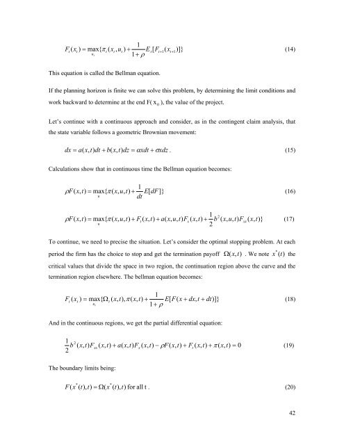
1Ft( xt) = max{ πt( xt, ut) + Et[Ft+1( xt+ 1)]}(14)ut1+ρThis equation is called the Bellman equation.If the planning horizon is finite we can solve this problem, by determining the limit conditions andwork backward to determine at the end F( x0), the value of the project.Let’s continue with a continuous approach and consider, as in the contingent claim analysis, thatthe state variable follows a geometric Brownian movement:dx = a( x,t)dt + b(x,t)dz = α xdt + σxdz. (15)Calculations show that in continuous time the Bellman equation becomes:1ρ F( x,t)= max{ π ( x,u,t)+ E[dF]}(16)udt1 2ρ F(x,t)= max{ π ( x,u,t)+ Ft( x,t)+ a(x,u,t)Fx( x,t)+ b ( x,u,t)Fxx(x,t)}(17)u2To continue, we need to precise the situation. Let’s consider the optimal stopping problem. At eachperiod the firm has the choice to stop and get the termination payoff Ω ( x,t). We note x * ( t ) thecritical values that divide the space in two region, the continuation region above the curve and thetermination region elsewhere. The bellman equation becomes:1Ft( xt) = max{ Ωt( x,t),π ( x,t)+ E[F(x + dx,t + dt)]}(18)ut1+ρAnd in the continuous regions, we get the partial differential equation:1 b 2 ( x , t ) F ( x , t ) + a ( x , t ) F ( x , t ) − F ( x , t ) + F ( x , t ) + ( x , t ) =xxxρtπ 0(19)2The boundary limits being:F(x**( t),t)= Ω(x ( t),t)for all t . (20)42