Managing Risks of Supply-Chain Disruptions: Dual ... - CiteSeerX

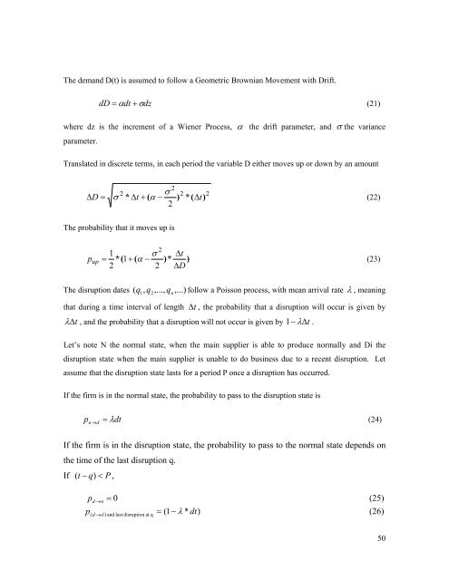
The demand D(t) is assumed to follow a Geometric Brownian Movement with Drift.dD = α dt + σdz(21)where dz is the increment of a Wiener Process, α the drift parameter, and σ the varianceparameter.Translated in discrete terms, in each period the variable D either moves up or down by an amount∆D=22 σ 2 2σ α(22)* ∆t+ ( − ) *( ∆t)2The probability that it moves up isp up21 σ ∆t= *( 1+( α − )* )(23)2 2 ∆DThe disruption dates q , q ,..., q ,...) follow a Poisson process, with mean arrival rate λ , meaning(1 2 nthat during a time interval of length∆ t , the probability that a disruption will occur is given byλ ∆t , and the probability that a disruption will not occur is given by 1 − λ∆t.Let’s note N the normal state, when the main supplier is able to produce normally and Di thedisruption state when the main supplier is unable to do business due to a recent disruption. Letassume that the disruption state lasts for a period P once a disruption has occurred.If the firm is in the normal state, the probability to pass to the disruption state isp n → d= λdt(24)If the firm is in the disruption state, the probability to pass to the normal state depends onthe time of the last disruption q.If ( t − q)< P ,p = 0(25)d →np( d → d ) and last disruption at q= (1 − λ * dt)(26)50