"Linear Equation Solver using CMOS Technology" - Microelectronic ...

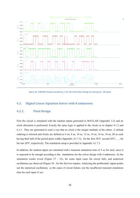
Figure 26. CADENCE Output waveforms_5 for the Final Solver Design (4 unknowns) - 30 inputs4.2. Digital Linear Equation Solver with 8 unknowns4.2.1. Final DesignFirst the circuit is simulated with the random inputs generated in MATLAB (Appendix 3.2) and noclock allocation is performed. Exactly the same logic is applied to the clocks as in chapter 4.1.2 and4.1.3 . They are generated in such a way that no clock is the integer multiple of the others. A defaultordering is selected and clocks are defined as 6 ns, 8 ns, 10 ns, 12 ns, 14 ns, 16 ns, 18 ns, 20 ns eachhaving their half of the period pulse width (Appendix A1.7.3), for the first DFF, second DFF, ... , forthe last DFF, respectively. The simulation setup is provided in Appendix A1.7.3.In addition, the random inputs are simulated with a transient simulation time of 5 us for each, since itis expected to be enough according to the simulations for the solver design with 4 unknowns. As thesimulation results reveal (Figure 27 - 32), for some input cases the circuit fails, and numericaloscillations are observed (Figure 30 - for the first two inputs). Analyzing the problematic inputs pointsout the numerical oscillations as the cause of circuit failure, not the insufficient transient simulationtime for each input (5 us).35