the humboldt current system of northern and central chile - figema

More documents

Recommendations

Info

MARTIN THIEL ET AL.appeared in June, and early developmental stages were found in the plankton until December (Palma1994), supporting the suggestion that reproduction is not synchronised among females. Gallardoet al. (1994) reported the first benthic stages in March with very high densities of recently settledsquat lobsters in April. Roa et al. (1995) identified nursery areas in places with very low oxygenconcentrations from where juveniles migrate to nearby adult habitats. It is generally assumed thatfemales produce only one clutch per year, but the extended reproductive period and the apparentlyshort incubation period of 2–3 months (Palma & Arana 1997) could allow some females to producemore than one clutch per year. Fecundity has been estimated at 1800–34,000 eggs in Region VIII(Palma & Arana 1997), and most females reach sexual maturity at carapace lengths of ~25 mm.Red squat lobsters are estimated to live from 5 to 10 yr (Roa & Tapia 1998).Biology and stock estimatesAs can be seen from the preceding section, information on the biology of the nylon shrimp andthe squat lobsters is mainly based on demographic data (size at first reproduction, fecundity, sexratio, per cent ovigerous females, embryo developmental stages), but little information is availableon their behaviour. A close analysis of monthly landings suggests possible seasonal changes inbehaviour during the year and indicates that it is important to incorporate this information in stockestimates (Pérez 2005).Pérez (2005) proposed that the biomass of the nylon shrimp showed well-defined cycles ofavailability (sensu Menge 1972), which were not related to its true abundance in biomass (sensuMenge 1972). The first cycle (termed the ‘short cycle’) occurs from September to December andis characterised by a decrease in availability (minimum in October), followed by a recovery(maximum availability in December). This leads to a cycle of greater length (termed the ‘longcycle’), characterised by a decline in available biomass, reaching a minimum in April and followedby an increase again reaching a maximum in August. Reasons for these cycles are not clear, but it hasbeen suggested that they are related to the moult and reproduction. In this sense, a sudden decreasein availability could be due to recently moulted individuals hiding from predators (Pérez 2005).The total biomass of Heterocarpus reedi in Region IV in September 1997 was estimated to beabout 5000 t, but not all of these shrimp were susceptible to fishing gear, resulting in an availablebiomass (to the fishery) of 4200 t (for details see Pérez 2005). The estimated total biomass decreasedto 2000 t in August 2000 (Week 143), representing a decline of 60% from that estimated at theinitiation of the simulation (Figure 25A). However, the percentage variation in the catch per uniteffort (CPUE) was not proportional to the decrease in abundance within periods of maximumavailability (Figure 25A). At the beginning of the study period, the CPUE was 0.59 t haul −1 , andin August 2000 this decreased to 0.45 t haul −1 , representing a decrease of only 24%. In recruitment,at each fishing station in 1997–1998 and 1998–1999 the difference between the control curves andavailability allowed the identification of two time windows for recruitment, one of lesser intensityin December and one of greater intensity extending through June and July. This seasonal variation inthe availability of the resource to the fishing gear has a direct influence on the population estimatesand consequently the determination of TACs. Therefore it was recommended to include this biologicalinformation in stock evaluation and to conduct the corresponding research cruises during periodsof maximum availability of the resource (Pérez 2005).Crustacean fisheries and economic considerationsFisheries respond not only to fluctuations in stock abundance but also to economic considerations.From the economic perspective, the annual TAC system has produced an increase in the fishing286
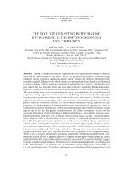
THE HUMBOLDT CURRENT SYSTEM OF NORTHERN AND CENTRAL CHILEBiomass (t)Million US$6000500040003000200010001997 1998 1999 2000Available biomassControl biomass00 20 40 60 80 100 120 140 160WeekA20Income7Costs1665124Cervimunida johni83Heterocarpus reedi241001997/98 1998/99 1999/00 1997/98 1998/99 1999/00Fishing seasonFigure 25 (A) Biomass dynamics of the nylon shrimp in Region IV. Available biomass is the biomass thatis available to the fishery and control biomass is the estimated total biomass of the resource according to themodel by Pérez (2005); bars above figure represent short cycles (light shading) and long cycles (dark shading)when resource becomes unavailable to fishery for biological reasons; for further details see text and reference.Weeks are numbered beginning with the week of 1 September 1997. (B) Comparison of total income withtotal costs by resource of crustacean trawl fishery in Region IV.Beffort, measured in terms of hauls, resulting in a decrease in the expected economic benefit basedon administrative measures. Pérez (2003) explored the bioeconomic effect produced by the decreasein CPUE in the nylon shrimp and yellow squat lobster fisheries in northern Chile during 1997–2000.A biological-technological simulation model was used by Pérez (2005), which took both physicaland biological variables into account. An economic submodel was incorporated into this model inorder to carry out an integrated analysis of the crustacean fisheries, which included the subsectorinvolving catches and their processing. The economic results obtained, when integrated with thecatch results and size of the stocks, allowed the dynamics of this fishery to be explained inRegions III and IV during 1997–2000, when the catch increased by 21%, and final productionincreased by 24% (measured as frozen tails), although the variable costs increased by only 11%(Figure 25B). In this same period the fisheries costs increased by 117% and the total productioncost increased by 93%. The results showed that part of the economic benefit was lost due to theeffect of a decrease in the biomasses of both resources and an excessive increase in the averageproduction costs (due to increased costs of fishing and extraction).This example underscores the importance of incorporating economic reference points in additionto biological (biomass) and fishery variables (CPUE and catch). Furthermore, basic biologicaldata (larval ecology, settlement biology, habitat requirements, seasonal migrations, and matingbehaviour) still need to be revealed for these three crustacean species. At present, very little is287
Page 1 and 2:
Oceanography and Marine Biology: An
Page 3 and 4:
THE HUMBOLDT CURRENT SYSTEM OF NORT
Page 5 and 6:
Page 7 and 8:
Page 9 and 10:
Page 11 and 12:
Page 13 and 14:
Page 15 and 16:
Page 17 and 18:
Page 19 and 20:
Page 21 and 22:
Page 23 and 24:
Page 25 and 26:
Page 27 and 28:
Page 29 and 30:
Page 31 and 32:
Page 33 and 34:
Page 35 and 36:
Page 37 and 38:
Page 39 and 40:
Page 41 and 42: THE HUMBOLDT CURRENT SYSTEM OF NORT
Page 91: THE HUMBOLDT CURRENT SYSTEM OF NORT
Page 143 and 144:
Page 145 and 146:
Page 147 and 148:
Page 149 and 150:
show all

the humboldt current system of northern and central chile - figema

You also want an ePaper? Increase the reach of your titles

Delete template?

Save as template?