Estimating the Water Requirements for Plants of Floodplain Wetlands

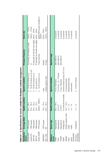
Table A1 – 2. Specifications for sensors suitable for floodplain wetland managementSpacebornesensorsCoverage dates Spatial resolution Spectral resolution Overpass frequency Scene sizeLandsat MSS 1972–present 80 m × 80 m 4 × 10–20 nm bands vis–nir 16 (currently, less frequent in past) 184 km × 172 kmLandsat TM 1982–present 30 m × 30 m 7 × 10–20 nm bands vis–nir–swir 16 184 km × 172 kmSPOT MS 1986–present 20 m × 20 m 3 × 10–20 nm bands vis–nir 26 days (less for off nadir view angles) 60 km × 60 kmSPOT Xs 1986–present 10 m × 10 m 1 × 25 nm band vis 27 days (less for off nadir view angles) 60 km × 60 kmNOAA AVHRR 1979–present 4000 m × 4000 m 4 × 10–20 nm bands vis–nir 7 days (nominal) global NDVI product available asCD-RomRADARSAT 1995–present 10 m × 10 m radar Flexible 50 km × 50 kmERS–1 SAR ??? 30 m × 30 m synthetic aperture radar 35 days 100 km × 100 kmAirbornesensorSensor type Spatial resolution Spectral resolution Spectral rangeAVIRIS Hyperspectral 20 m × 20 m 10 nm, 224 bands 400–2500 nm as acquiredCASI Hyperspectral 0.8–5 m 2 2.2 nm min., 10 – 72 bands 400–1000 nm as acquiredHYMAP Hyperspectral 2–10 m 2 16 nm, 128 bands 400–2500 nm as acquiredLIDAR Profiling laser 3 m intervals horizontally minimum vertical accuracy 10–15 cm as acquiredAIRSAR Synthetic aperture radar 10 m × 10 m 3 microwave bands as acquiredVideo visible 1 m × 1 m filtered panchromatic as acquiredAerialphotographyvisible 1 m × 1 m panchromatic as acquiredCIR Aerialphotographymultispectral 1 m × 1 m 3 × 10–20 nm bands as acquiredAppendix 1: Remote Sensing 103