Estimating the Water Requirements for Plants of Floodplain Wetlands

More documents

Recommendations

Info

Table A1 – 4. A flooding overlay checkInundation area for three flood events on the Gwydir River, 1975 to 1983. Agreement between flood events,indicated by the area of overlap and non-overlap, was low, and was not dependent on flood size. Reasons for thiswere not determined at the time the analysis was done, but this was a period of floodplain development (Roberts,unpublished data).Event size Area of overlap Area of non-overlap150 GL a month and 130 GL month 11,033 ha 6,0001 (35.2%) of smaller flood not flooded by larger flood150 GL month and 303 GL month 29,801 ha 7,935 ha (21.0%) of smaller flood not flooded by larger flood130 GL month and 303 GL month 13,580 ha 3,474 ha (20.4%) of smaller flood not flooded by larger flooda GL = gigalitre = 1,000,000,000 litresTable A1 – 5. Comparison of two methodsInundated area estimated for three floods using two methods of interpretation: Method 1, visual interpretation offlooded area on hard copy, measured by planimetry; Method 2, micro-BRIAN estimated flooded areas afterrectifying grey-scale images, using scanned and digitised hard copy (Roberts, unpublished data).Date of image Method 1 Method 2 Change as %, as area (ha)1 November 1975 37,500 37,736
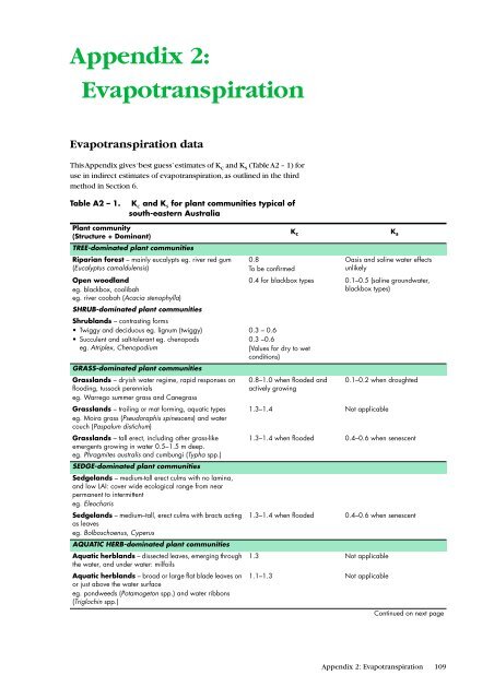
Appendix 2:EvapotranspirationEvapotranspiration dataThis Appendix gives ‘best guess’ estimates of K c and K s (Table A2 – 1) foruse in indirect estimates of evapotranspiration, as outlined in the thirdmethod in Section 6.Table A2 – 1.K c and K s for plant communities typical ofsouth-eastern AustraliaPlant community(Structure + Dominant)TREE-dominated plant communitiesRiparian forest – mainly eucalypts eg. river red gum(Eucalyptus camaldulensis)Open woodlandeg. blackbox, coolibaheg. river coobah (Acacia stenophylla)SHRUB-dominated plant communitiesShrublands – contrasting forms• Twiggy and deciduous eg. lignum (twiggy)• Succulent and salt-tolerant eg. chenopodseg. Atriplex, ChenopodiumGRASS-dominated plant communitiesGrasslands – dryish water regime, rapid responses onflooding, tussock perennialseg. Warrego summer grass and CanegrassGrasslands – trailing or mat forming, aquatic typeseg. Moira grass (Pseudoraphis spinescens) and watercouch (Paspalum distichum)Grasslands – tall erect, including other grass-likeemergents growing in water 0.5–1.5 m deep.eg. Phragmites australis and cumbungi (Typha spp.)SEDGE-dominated plant communitiesSedgelands – medium-tall erect culms with no lamina,and low LAI: cover wide ecological range from nearpermanent to intermittenteg. EleocharisSedgelands – medium–tall, erect culms with bracts actingas leaveseg. Bolboschoenus, CyperusAQUATIC HERB-dominated plant communitiesAquatic herblands – dissected leaves, emerging throughthe water, and under water: milfoilsAquatic herblands – broad or large flat blade leaves onor just above the water surfaceeg. pondweeds (Potamogeton spp.) and water ribbons(Triglochin spp.)K c0.8To be confirmedK sOasis and saline water effectsunlikely0.4 for blackbox types 0.1–0.5 (saline groundwater,blackbox types)0.3 – 0.60.3 –0.6(Values for dry to wetconditions)0.8–1.0 when flooded andactively growing0.1–0.2 when droughted1.3–1.4 Not applicable1.3–1.4 when flooded 0.4–0.6 when senescent1.3–1.4 when flooded 0.4–0.6 when senescent1.3 Not applicable1.1–1.3 Not applicableContinued on next pageAppendix 2: Evapotranspiration 109
Page 1 and 2:
Estimating the WaterRequirements fo
Page 3 and 4:
ContentsPreface 7Acknowledgments 8G
Page 5:
List of Tables1 Spatial variability
Page 8 and 9:
Note that the guide is concerned pr
Page 10 and 11:
ecomes a matter of how to use what
Page 12 and 13:
Figure 1. Floodplain featuresThe fl
Page 14 and 15:
Figure 4.Wanganella Swamps, souther
Page 16 and 17:
Floodplain wetlands, being a mosaic
Page 18 and 19:
Section 2:Introducing theVegetation
Page 20 and 21:
size and vigour rarely reach their
Page 22 and 23:
floodplains survive there because t
Page 24 and 25:
The lagoon floor is then colonised
Page 26 and 27:
Note 11Growth-formsField guides to
Page 28 and 29:
identical conditions. PFTs differ f
Page 30 and 31:
Note 13Changes in depthSome herbace
Page 32 and 33:
Focusing on depthWater regime analy
Page 34 and 35:
Note 15Internet dataEnvironmental d
Page 36 and 37:
Step 3: Vegetation-hydrologyrelatio
Page 38 and 39:
Note 19Modelling and time-stepsIn s
Page 40 and 41:
Section 4: Old andNew DataOne of th
Page 42 and 43:
see Figure 15), despite a three-fol
Page 44 and 45:
frequency. This is rather limiting,
Page 46 and 47:
Figure 13. Lippia, a floodplain wee
Page 48 and 49:
single measure of the vegetation to
Page 50 and 51:
Section 5:ObtainingVegetation DataW
Page 52 and 53:
However, if the chosen species has
Page 54 and 55:
Figure 15. Range of tree condition
Page 56 and 57:
Figure 16. Spatial-temporal sequenc
Page 58 and 59: Note 26Canopy condition indexA visu
Page 60 and 61: Note 27Mapping floodplainwetland ve
Page 62 and 63: Shape of species responseThe shape
Page 64 and 65: Figure 18. Heat pulse sensorHeat pu
Page 66 and 67: section, using storage volume and i
Page 68 and 69: Figure 20. Crack volume and drying
Page 70 and 71: Figure 21. The relationshipbetween
Page 72 and 73: epresentative, there should be no m
Page 74 and 75: All of the curves are described by
Page 76 and 77: monitoring, precision levels, scali
Page 78 and 79: sites of significant recharge and d
Page 80 and 81: Figure 24. Degraded channelPart of
Page 82 and 83: and so depth estimates are inaccura
Page 84 and 85: Section 7:PredictingVegetationRespo
Page 86 and 87: AEAM and the Macquarie Marshes. An
Page 88 and 89: Category 3: hydraulic/empiricalAppr
Page 90 and 91: For example, changes in surface and
Page 92 and 93: ReferencesPrefaceArthington AH and
Page 94 and 95: Section 3Roberts J and Marston F (1
Page 96 and 97: Kunin WE and Gaston KG (1993). The
Page 98 and 99: Singh VP (1995).“Computer models
Page 100 and 101: Web ListingsNote 40Data on the WebM
Page 102 and 103: flood. This has not been attempted,
Page 104 and 105: Seven points over the flow range is
Page 106 and 107: used as exclusions; or can be quant
Page 110: Table A2 - 1.(cont’d) K c and K s
show all

Estimating the Water Requirements for Plants of Floodplain Wetlands

You also want an ePaper? Increase the reach of your titles

Delete template?

Save as template?