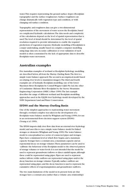
Figure 24. Degraded channelPart <strong>of</strong> <strong>the</strong> lower Gwydir floodplainshowing a flood runner which has cutdown; <strong>the</strong> banks and <strong>the</strong> floodplainare mainly covered with lippia. Thistype <strong>of</strong> erosion limits <strong>the</strong> spread <strong>of</strong>floodwater and can invalidatevolume–inundation area relationships.Photo taken in dry conditions, in1993.Modelling wetland water balanceOnce a time series <strong>for</strong> each inflow and outflow (or at least <strong>the</strong> dominantinflows and outflows) has been established <strong>for</strong> a matching period,prediction <strong>of</strong> changes in storage volume <strong>of</strong> <strong>the</strong> wetland through time ispossible. This constitutes a model <strong>of</strong> <strong>the</strong> wetland water balance.Because each time series is likely to contain some degree <strong>of</strong> error, it isdesirable to validate <strong>the</strong> model using independent estimates <strong>of</strong> storagevolumes. In cases where <strong>the</strong> inflow and outflows have all beenestimated directly from hydrologic, climatic and vegetation data (<strong>for</strong>instance river inflows and evapotranspiration outflows), images <strong>of</strong>inundation areas <strong>for</strong> different floods will provide an independent meansto validate <strong>the</strong> water balance model.A water-balance model can be used not only to explain past hydrologicbehaviour but also to predict future hydrologic behaviour under alteredconditions. For example, a model may be used to determine <strong>the</strong>impacts on storage volumes <strong>of</strong> an altered river flood regime. A modelmay also be used to predict <strong>the</strong> impacts <strong>of</strong> imposed changes in <strong>the</strong>vegetation, such as <strong>the</strong> changes in storage volume that would resultfrom <strong>the</strong> removal <strong>of</strong> large trees from a floodplain. A discussion <strong>of</strong>catchment and river hydrology modelling techniques is beyond <strong>the</strong>scope <strong>of</strong> this guide (Note 38).Spatial variability. <strong>Floodplain</strong> wetlands that have variable topographyand soils will also have variable water regime and vegetation. Thisspatial variability must be recognised. Little can usefully be said about<strong>the</strong> expected vegetation response if <strong>the</strong> wetland is considered as anentity, represented by a spatially averaged water regime. Instead, waterbalance calculations should be undertaken on sub-components <strong>of</strong> <strong>the</strong>floodplain wetland. These sub-components should be areas that havenearly uni<strong>for</strong>m hydrologic behaviour; examples are surface depressionswith similar flooding and retention characteristics; or floodplainterraces with similar flood frequency and duration characteristics andsimilar vegetation roughness.Note 38Catchment modellingTo understand <strong>the</strong> ma<strong>the</strong>maticaltechniques used in modellingrainfall–run-<strong>of</strong>f process, overlandflow and channel flow, see a generalintroductory hydrology text; <strong>for</strong>example, “Physical hydrology”(Dingman 1994). For more about<strong>the</strong> available models <strong>of</strong> catchmenthydrology see “Computer models inwatershed hydrology” (Singh 1995)and <strong>for</strong> floodplain hydrology andhydraulics see “Computer-assistedfloodplain hydrology and hydraulics”(Hoggan 1996).If aiming to restore <strong>the</strong> ‘natural’ water regime, it is less important tounderstand spatial variability than in <strong>the</strong> case <strong>of</strong> rehabilitation, where aprediction <strong>of</strong> <strong>the</strong> vegetation response is required.<strong>Water</strong> movements. In low relief environments, such as lowland riverfloodplains, water moves relatively slowly and is strongly influenced bysurface roughness. <strong>Water</strong>-balance calculations do not consider flowresistance, so may give a poor indication <strong>of</strong> how water moves and isdistributed across <strong>the</strong> floodplain. For accurate predictions <strong>of</strong> this overshort time steps, modelling water movement will be required. Forexample, if <strong>the</strong> topography and roughness <strong>of</strong> <strong>the</strong> floodplain are suchthat surface water flows at speeds <strong>of</strong> a few centimetres per second(equivalent to hundreds <strong>of</strong> metres per day), <strong>the</strong>n to predict <strong>the</strong> dailydistribution <strong>of</strong> water across a floodplain many kilometres in extent willrequire consideration <strong>of</strong> flow velocities and hence surface roughness.However, if it is only necessary to predict <strong>the</strong> monthly distribution <strong>of</strong>water, water-balance calculations and a consideration <strong>of</strong> <strong>the</strong> topographywill be sufficient.Modelling flow velocity requires a hydraulic, ra<strong>the</strong>r than a hydrological,perspective. Modelling <strong>the</strong> hydraulics <strong>of</strong> a floodplain wetland accounts<strong>for</strong> <strong>the</strong> energy involved in <strong>the</strong> surface flows, not just <strong>the</strong> volumes <strong>of</strong>80 <strong>Estimating</strong> <strong>the</strong> <strong>Water</strong> <strong>Requirements</strong> <strong>for</strong> <strong>Plants</strong> <strong>of</strong> <strong>Floodplain</strong> <strong>Wetlands</strong>
water. This requires representing <strong>the</strong> ground surface slopes (floodplaintopography) and <strong>the</strong> surface roughnesses. Surface roughness canchange dramatically with vegetation type and condition, or withchanging soil surface condition.Topographic and roughness data can give a two-dimensionalrepresentation <strong>of</strong> <strong>the</strong> movement <strong>of</strong> water across <strong>the</strong> floodplain, basedon complicated hydraulic calculations. The data needs and complexity<strong>of</strong> <strong>the</strong> calculations depend on <strong>the</strong> level <strong>of</strong> spatial representation that isused. The level <strong>of</strong> detail should be determined by <strong>the</strong> level <strong>of</strong> spatialresolution required to provide in<strong>for</strong>mation to enable <strong>the</strong> requiredpredictions <strong>of</strong> vegetation response. Hydraulic modelling <strong>of</strong> floodplains isa major undertaking, usually based on complex computer modellingusing large data sets. Accurate calibration or even validation <strong>of</strong> suchmodels is <strong>of</strong>ten constrained by <strong>the</strong> lack <strong>of</strong> appropriate data to describefloodplain water movement.Australian examplesFive Australian examples <strong>of</strong> wetland or floodplain hydrology modellingare described below, all from <strong>the</strong> Murray–Darling Basin. The first is asimple water balance approach. The second is an empirical model basedon relating river levels to inundation imagery. The third and four<strong>the</strong>xamples are <strong>of</strong> hydraulic floodplain modelling: one <strong>of</strong> <strong>the</strong> lowerMacintyre River floodplain by Connell Wagner (Qld) Pty Ltd, <strong>the</strong> o<strong>the</strong>r<strong>of</strong> Condamine–Balonne River floodplain by <strong>the</strong> Snowy MountainsEngineering Corporation (SMEC) (Marr 1999). The last exampledescribes <strong>the</strong> range <strong>of</strong> different wetland and floodplain modellingapproaches used in <strong>the</strong> IQQM river hydrology model developed by <strong>the</strong>NSW Department Land and <strong>Water</strong> Conservation.EFDSS and <strong>the</strong> Murray–Darling BasinOne <strong>of</strong> <strong>the</strong> simplest approaches to representing water movementthrough a wetland complex was taken in <strong>the</strong> development <strong>of</strong> afloodplain water balance model by Whigham and Young (1999), <strong>for</strong> usein an environmental flows decision support system (EFDSS)(Young et al. 1999).The EFDSS imports daily river flow data from an external river hydrologymodel, and uses this to run a simple water balance model <strong>for</strong> linkedstorages or elements (Whigham and Young 1999). The water balancemodel is conceptualised as a series <strong>of</strong> connected pipes and storages.Pipes have a minimum level at which flow begins, and a maximumcapacity. Storages have a constant area, a maximum capacity and anexponential decay on storage volumes. These parameters can be used to‘calibrate’ <strong>the</strong> behaviour <strong>of</strong> <strong>the</strong> floodplain model to <strong>the</strong> observed pattern<strong>of</strong> storage volumes or water levels. It is not intended that <strong>the</strong> model beused to represent groundwater inflows or direct rainfall inputs, although<strong>the</strong>se could be represented using pipes. Pipes are used to representsurface inflows: while outflows are represented using pipes and/or <strong>the</strong>decay function on storage volumes. Typically, surface outflows arerepresented using pipes, and <strong>the</strong> decay function is used to represent <strong>the</strong>cumulative effects <strong>of</strong> evapotranspiration and groundwater outflows.The two main limitations <strong>of</strong> <strong>the</strong> model in its present <strong>for</strong>m are thatstorages have a constant area (ra<strong>the</strong>r than a volume–area relationship)Section 6: Using <strong>Water</strong> Regime Data 81
- Page 1 and 2:
Estimating the WaterRequirements fo
- Page 3 and 4:
ContentsPreface 7Acknowledgments 8G
- Page 5:
List of Tables1 Spatial variability
- Page 8 and 9:
Note that the guide is concerned pr
- Page 10 and 11:
ecomes a matter of how to use what
- Page 12 and 13:
Figure 1. Floodplain featuresThe fl
- Page 14 and 15:
Figure 4.Wanganella Swamps, souther
- Page 16 and 17:
Floodplain wetlands, being a mosaic
- Page 18 and 19:
Section 2:Introducing theVegetation
- Page 20 and 21:
size and vigour rarely reach their
- Page 22 and 23:
floodplains survive there because t
- Page 24 and 25:
The lagoon floor is then colonised
- Page 26 and 27:
Note 11Growth-formsField guides to
- Page 28 and 29:
identical conditions. PFTs differ f
- Page 30 and 31: Note 13Changes in depthSome herbace
- Page 32 and 33: Focusing on depthWater regime analy
- Page 34 and 35: Note 15Internet dataEnvironmental d
- Page 36 and 37: Step 3: Vegetation-hydrologyrelatio
- Page 38 and 39: Note 19Modelling and time-stepsIn s
- Page 40 and 41: Section 4: Old andNew DataOne of th
- Page 42 and 43: see Figure 15), despite a three-fol
- Page 44 and 45: frequency. This is rather limiting,
- Page 46 and 47: Figure 13. Lippia, a floodplain wee
- Page 48 and 49: single measure of the vegetation to
- Page 50 and 51: Section 5:ObtainingVegetation DataW
- Page 52 and 53: However, if the chosen species has
- Page 54 and 55: Figure 15. Range of tree condition
- Page 56 and 57: Figure 16. Spatial-temporal sequenc
- Page 58 and 59: Note 26Canopy condition indexA visu
- Page 60 and 61: Note 27Mapping floodplainwetland ve
- Page 62 and 63: Shape of species responseThe shape
- Page 64 and 65: Figure 18. Heat pulse sensorHeat pu
- Page 66 and 67: section, using storage volume and i
- Page 68 and 69: Figure 20. Crack volume and drying
- Page 70 and 71: Figure 21. The relationshipbetween
- Page 72 and 73: epresentative, there should be no m
- Page 74 and 75: All of the curves are described by
- Page 76 and 77: monitoring, precision levels, scali
- Page 78 and 79: sites of significant recharge and d
- Page 82 and 83: and so depth estimates are inaccura
- Page 84 and 85: Section 7:PredictingVegetationRespo
- Page 86 and 87: AEAM and the Macquarie Marshes. An
- Page 88 and 89: Category 3: hydraulic/empiricalAppr
- Page 90 and 91: For example, changes in surface and
- Page 92 and 93: ReferencesPrefaceArthington AH and
- Page 94 and 95: Section 3Roberts J and Marston F (1
- Page 96 and 97: Kunin WE and Gaston KG (1993). The
- Page 98 and 99: Singh VP (1995).“Computer models
- Page 100 and 101: Web ListingsNote 40Data on the WebM
- Page 102 and 103: flood. This has not been attempted,
- Page 104 and 105: Seven points over the flow range is
- Page 106 and 107: used as exclusions; or can be quant
- Page 108 and 109: Table A1 - 4. A flooding overlay ch
- Page 110: Table A2 - 1.(cont’d) K c and K s