- Page 2:
TEXTILE COMPOSITES AND INFLATABLE S
- Page 6:
Textile Composites and Inflatable S
- Page 10:
Table of Contents Preface .........
- Page 14:
PREFACE The objective of this book
- Page 18:
2 Rosemarie Wagner can be evaluated
- Page 22:
4 Rosemarie Wagner The tension forc
- Page 26:
6 Rosemarie Wagner The tension stre
- Page 30:
8 Rosemarie Wagner Fig. 10. Model d
- Page 34:
10 Rosemarie Wagner Fig. 12. Influe
- Page 38:
12 Rosemarie Wagner Length Lx x = L
- Page 42:
14 Rosemarie Wagner net with triang
- Page 46:
16 Rosemarie Wagner 7. Bletzinger K
- Page 50:
18 Erik Moncrieff Structural Engine
- Page 54:
20 Erik Moncrieff are, by definitio
- Page 58:
22 Erik Moncrieff 3 Modelling Texti
- Page 62:
24 Erik Moncrieff which seek to mod
- Page 66:
26 Erik Moncrieff high level optimi
- Page 70:
28 Erik Moncrieff Developments in c
- Page 74:
30 Lothar Grundig, ¨ Dieter Str¨
- Page 78:
32 Lothar Grundig, ¨ Dieter Str¨
- Page 82:
34 Lothar Grundig, ¨ Dieter Str¨
- Page 86:
36 Lothar Grundig, ¨ Dieter Str¨
- Page 90:
38 Lothar Grundig, ¨ Dieter Str¨
- Page 94:
40 Lothar Grundig, ¨ Dieter Str¨
- Page 98:
42 Lothar Grundig, ¨ Dieter Str¨
- Page 102:
44 Lothar Grundig, ¨ Dieter Str¨
- Page 106:
Finite Element Analysis of Membrane
- Page 110:
Finite Element Analysis of Membrane
- Page 114:
Finite Element Analysis of Membrane
- Page 118:
Finite Element Analysis of Membrane
- Page 122:
x 1 Finite Element Analysis of Memb
- Page 126:
and Finite Element Analysis of Memb
- Page 130:
Finite Element Analysis of Membrane
- Page 134:
6 Numerical Examples Finite Element
- Page 138:
Finite Element Analysis of Membrane
- Page 142:
6.4 Inflation of a Balloon Finite E
- Page 146:
7Closure Finite Element Analysis of
- Page 150:
Applications of a Rotation-Free Tri
- Page 154:
2 3 Applications of a Rotation-Free
- Page 158:
Applications of a Rotation-Free Tri
- Page 162:
Applications of a Rotation-Free Tri
- Page 166:
in Applications of a Rotation-Free
- Page 170:
(a) DIAPHRAGM α =40 300 SYMMETRY Z
- Page 174:
Applications of a Rotation-Free Tri
- Page 178:
Applications of a Rotation-Free Tri
- Page 182:
Applications of a Rotation-Free Tri
- Page 186:
Applications of a Rotation-Free Tri
- Page 190:
FE Analysis of Membrane Systems Inc
- Page 194:
FE Analysis of Membrane Systems Inc
- Page 198:
FE Analysis of Membrane Systems Inc
- Page 202:
FE Analysis of Membrane Systems Inc
- Page 206:
FE Analysis of Membrane Systems Inc
- Page 210:
FE Analysis of Membrane Systems Inc
- Page 214:
FE Analysis of Membrane Systems Inc
- Page 218:
FE Analysis of Membrane Systems Inc
- Page 222:
FE Analysis of Membrane Systems Inc
- Page 226:
FE Analysis of Membrane Systems Inc
- Page 230:
Wrinkles in Square Membranes Y.W. W
- Page 234:
Wrinkles in Square Membranes 111 ra
- Page 238:
1 R T 2=T 1 T 1 =T 2 L T1 =T2 L (a)
- Page 242:
R wrin -r 1 R r 1 w θ r Wrinkles i
- Page 246:
Wrinkles in Square Membranes 117 fo
- Page 250:
C (b) B Wrinkles in Square Membrane
- Page 254:
Wrinkles in Square Membranes 121 by
- Page 258:
F.E.M. for Prestressed Saint Venant
- Page 262:
F.E.M. for Prestressed Saint Venant
- Page 266:
with: F.E.M. for Prestressed Saint
- Page 270: F.E.M. for Prestressed Saint Venant
- Page 274: F.E.M. for Prestressed Saint Venant
- Page 278: F.E.M. for Prestressed Saint Venant
- Page 282: F.E.M. for Prestressed Saint Venant
- Page 286: OY axis (in) F.E.M. for Prestressed
- Page 290: F.E.M. for Prestressed Saint Venant
- Page 294: F.E.M. for Prestressed Saint Venant
- Page 298: Equilibrium Consistent Anisotropic
- Page 302: Equilibrium Consistent Anisotropic
- Page 306: Equilibrium Consistent Anisotropic
- Page 310: 5 Equilibrium Consistent Anisotropi
- Page 314: Equilibrium Consistent Anisotropic
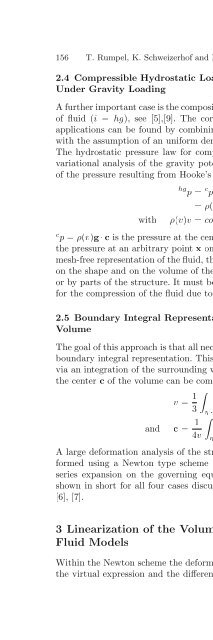
- Page 318: 154 T. Rumpel, K. Schweizerhof and
- Page 324: FE Modelling and Simulation of Gas
- Page 328: FE Modelling and Simulation of Gas
- Page 332: FE Modelling and Simulation of Gas
- Page 336: FE Modelling and Simulation of Gasa
- Page 340: FE Modelling and Simulation of Gas
- Page 344: FE Modelling and Simulation of Gas
- Page 348: FE Modelling and Simulation of Gas
- Page 352: FE Modelling and Simulation of Gas
- Page 356: Widespan Membrane Roof Structures:
- Page 360: Widespan Membrane Roof Structures 1
- Page 364: Widespan Membrane Roof Structures 1
- Page 368: Widespan Membrane Roof Structures 1
- Page 372:
Widespan Membrane Roof Structures 1
- Page 376:
Widespan Membrane Roof Structures 1
- Page 380:
Widespan Membrane Roof Structures 1
- Page 384:
3 Reliability Analysis Widespan Mem
- Page 388:
Widespan Membrane Roof Structures 1
- Page 392:
4 Monitoring Widespan Membrane Roof
- Page 396:
Widespan Membrane Roof Structures 1
- Page 400:
Fabric Membranes Cutting Pattern Be
- Page 404:
2.2 Geometrical Issues Fabric Membr
- Page 408:
3 Cutting Shapes Determination 3.1
- Page 412:
3.2 Stress Composition Method Fabri
- Page 416:
Fabric Membranes Cutting Pattern 20
- Page 420:
Fabric Membranes Cutting Pattern 20
- Page 424:
Fabric Membranes Cutting Pattern 20
- Page 428:
Fabric Membranes Cutting Pattern 20
- Page 432:
curvatures are hence: Fabric Membra
- Page 436:
Inflated Membrane Structures on the
- Page 440:
Inflated Membrane Structures on the
- Page 444:
Inflated Membrane Structures on the
- Page 448:
Inflated Membrane Structures on the
- Page 452:
Post-Tensioned Modular Inflated Str
- Page 456:
Post-Tensioned Modular Inflated Str
- Page 460:
Post-Tensioned Modular Inflated Str
- Page 464:
Post-Tensioned Modular Inflated Str
- Page 468:
5 Technological Concepts 5.1 Air-In
- Page 472:
Post-Tensioned Modular Inflated Str
- Page 476:
6 Examples of Application Post-Tens
- Page 480:
Post-Tensioned Modular Inflated Str
- Page 484:
Post-Tensioned Modular Inflated Str
- Page 488:
7Conclusive Remarks Post-Tensioned
- Page 492:
242 Javier Marcipar, Eugenio Oñate
- Page 496:
244 Javier Marcipar, Eugenio Oñate
- Page 500:
246 Javier Marcipar, Eugenio Oñate
- Page 504:
248 Javier Marcipar, Eugenio Oñate
- Page 508:
250 Javier Marcipar, Eugenio Oñate
- Page 512:
252 Javier Marcipar, Eugenio Oñate
- Page 516:
254 Javier Marcipar, Eugenio Oñate
- Page 520:
256 Javier Marcipar, Eugenio Oñate
- Page 524:
Recent Advances in the Rigidization
- Page 528:
Recent Advances in the Rigidization
- Page 532:
Recent Advances in the Rigidization
- Page 536:
Recent Advances in the Rigidization
- Page 540:
Recent Advances in the Rigidization
- Page 544:
Recent Advances in the Rigidization
- Page 548:
Technology Evaluation Recent Advanc
- Page 552:
Recent Advances in the Rigidization
- Page 556:
Absorbance 0,5 0,4 0,3 0,2 0,1 Rece
- Page 560:
Recent Advances in the Rigidization
- Page 564:
Recent Advances in the Rigidization
- Page 568:
Recent Advances in the Rigidization
- Page 572:
Recent Advances in the Rigidization
- Page 576:
286 Edgar Stach Key words: Form-opt
- Page 580:
288 Edgar Stach 3 2-D Bubble Cluste
- Page 584:
290 Edgar Stach Fig. 15. Closest pa
- Page 588:
292 Edgar Stach Fig. 17. Various ge
- Page 592:
294 Edgar Stach Fig. 20. SKO method
- Page 596:
296 Edgar Stach Fig. 26. Fig. 27. D
- Page 600:
298 Edgar Stach Fullerene 5 The sma
- Page 604:
300 Edgar Stach To take Fuller’s
- Page 608:
302 Edgar Stach Figs. 47-49. The me
- Page 612:
Making Blobs with a Textile Mould A
- Page 616:
Making Blobs with aTextile Mould 30
- Page 620:
Making Blobs with aTextile Mould 30
- Page 624:
Fig. 11. Bending for power, a pole
- Page 628:
Making Blobs with aTextile Mould 31
- Page 632:
Making Blobs with aTextile Mould 31
- Page 636:
Fig. 30. To create a declining faca
- Page 640:
Making Blobs with aTextile Mould 31
- Page 644:
7Conclusion Making Blobs with aText