Ejercicios Resueltos de Estadística: Tema 2 ... - Academia Diego

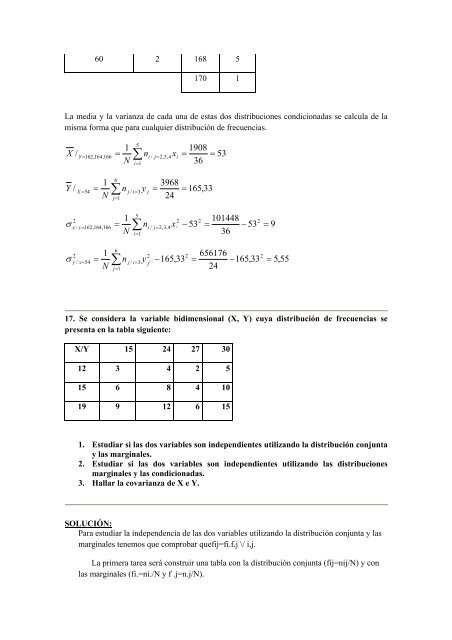
60 2 168 5170 1La media y la varianza de cada una de estas dos distribuciones condicionadas se calcula de lamisma forma que para cualquier distribución de frecuencias.X /Y /51= ∑ nN1908=36Y = 162 ,164,166i / j=2,3,4xi=i=161= ∑ nN3968=24X = 54 j / i=3yj=j=1165,33521 2 2 101448 2σx / y=162,164,166= ∑ ni/ j=2,3,4xi − 53 = − 53 = 9N36i=162 1 22 6561762σy / x=54= ∑ nj / i=3y i −165,33= −165,33= 5,55jN24j=15317. Se considera la variable bidimensional (X, Y) cuya distribución de frecuencias sepresenta en la tabla siguiente:X/Y 15 24 27 3012 3 4 2 515 6 8 4 1019 9 12 6 151. Estudiar si las dos variables son independientes utilizando la distribución conjuntay las marginales.2. Estudiar si las dos variables son independientes utilizando las distribucionesmarginales y las condicionadas.3. Hallar la covarianza de X e Y.SOLUCIÓN:Para estudiar la independencia de las dos variables utilizando la distribución conjunta y lasmarginales tenemos que comprobar quefij=fi.f.j \/ i,j.La primera tarea será construir una tabla con la distribución conjunta (fij=nij/N) y conlas marginales (fi.=ni./N y f .j=n.j/N).