Introduction à la théorie des poutres - mms2 - MINES ParisTech
Introduction à la théorie des poutres - mms2 - MINES ParisTech
Introduction à la théorie des poutres - mms2 - MINES ParisTech

Create successful ePaper yourself
Turn your PDF publications into a flip-book with our unique Google optimized e-Paper software.
Expression <strong>des</strong> contraintes locales<br />
Connaissant x 1 → (U, V , θ) ∀ x 1 ∈ [0, L], il est possible de calculer ε ∼<br />
(u) et d’en déduire σ ∼<br />
en<br />
utilisant <strong>la</strong> loi de comportement de <strong>la</strong> théorie générale <strong>des</strong> milieux continus.<br />
⎛<br />
( ) ⎜<br />
U ,1 + θ ,1 x 3 0<br />
ε.. = ⎝<br />
V ,1 +θ<br />
2<br />
0 0 0<br />
V ,1 +θ<br />
2 0 0<br />
⎞<br />
⎟<br />
⎠ (30)<br />
On obtient en particulier :<br />
σ 11 = E (U ,1 + θ ,1 x 3 )<br />
⇒ σ 11 = N S + M I<br />
x 3<br />
Le maximum de contrainte est obtenu au point le plus éloigné en x 3 de <strong>la</strong> ligne moyenne. Ce point<br />
a pour coordonnée x 3 = ρ :<br />
max<br />
(x 2 , x 3 )∈S σ 11 = N S + M I<br />
ρ<br />
MMS 2012, Contraintes locales <strong>Introduction</strong> à <strong>la</strong> théorie <strong>des</strong> <strong>poutres</strong> 21/28