Blaga P. Lectures on the differential geometry of - tiera.ru

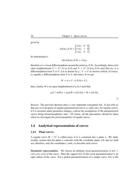
26 Chapter 1. Space curves
given by
Its determinant is
⎡
x
J(ψ)(t0, 0, 0) = ⎢⎣
′ (t0) 0 0
y ′ (t0) 1 0
z ′ ⎤
⎥⎦
(t0) 0 1
det J(ψ)(t0, 0, 0) = x ′ (t0),
therefore ψ is a local diffeomorphism around the point (t0, 0, 0). Accordingly, there exist
open neighborhoods U ⊂ R 3 of (t0, 0, 0) and V ⊂ R 3 of ψ(t0, 0, 0) such that ψ|V is a
diffeomorphism from U to V. Let us denote by ϕ : V → U its inverse (which, of course,
is, equally, a diffeomorphism from V to U, this time). If we put
W := {t ∈ I : (t, 0, 0) ∈ U} ,
then, clearly, W is an open neighborhood of t0 in I such that
ϕ(V ∩ r(W)) = ϕ(ψ(W × {(0, 0)}) = W × {(0, 0)}.
Remark. The previous theorem plays a very important conceptual role. It just tells us
that any local property of regular parameterized curves is valid, also, for regular curves,
if it is invariant under parameter changes, without the assumptions of the parameterized
curves being homeomorphisms onto. Of course, all the precautions should be taken
when we investigate the global properties of regular curves.
1.4 Analytical representations of curves
1.4.1 Plane curves
A regular curve M ⊂ R 3 is called plane if it is contained into a plane π. We shall,
usually, assume that the plane π coincides with the coordinate plane xOy and we shall
use, therefore, only the coordinates x and y to describe such curves.
Parametric representation. We choose an arbitrary local parameterization (I, r(t) =
(x(t), y(t), z(t))) of the curve. Then the support r(I) of this local parameterization is an
open subset of the curve. For a global parameterization of a simple curve, r(I) is the
�