Blaga P. Lectures on the differential geometry of - tiera.ru
Blaga P. Lectures on the differential geometry of - tiera.ru
Blaga P. Lectures on the differential geometry of - tiera.ru

Create successful ePaper yourself
Turn your PDF publications into a flip-book with our unique Google optimized e-Paper software.
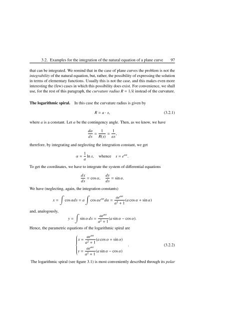
3.2. Examples for <strong>the</strong> integrati<strong>on</strong> <strong>of</strong> <strong>the</strong> natural equati<strong>on</strong> <strong>of</strong> a plane curve 97<br />
that can be integrated. We remind that in <strong>the</strong> case <strong>of</strong> plane curves <strong>the</strong> problem is not <strong>the</strong><br />
integrability <strong>of</strong> <strong>the</strong> natural equati<strong>on</strong>, but, ra<strong>the</strong>r, <strong>the</strong> possibility <strong>of</strong> expressing <strong>the</strong> soluti<strong>on</strong><br />
in terms <strong>of</strong> elementary functi<strong>on</strong>s. Usually this is not <strong>the</strong> case, and this makes even more<br />
interesting <strong>the</strong> (few) cases in which this possibility does exist. For c<strong>on</strong>venience, we shall<br />
use, for <strong>the</strong> rest <strong>of</strong> this paragraph, <strong>the</strong> curvature radius R = 1/k instead <strong>of</strong> <strong>the</strong> curvature.<br />
The logarithmic spiral. In this case <strong>the</strong> curvature radius is given by<br />
R = a · s, (3.2.1)<br />
where a is a c<strong>on</strong>stant. Let α be <strong>the</strong> c<strong>on</strong>tingency angle. Then, as we know, we have<br />
dα<br />
ds<br />
1 1<br />
= =<br />
R(s) as ,<br />
<strong>the</strong>refore, by integrating and neglecting <strong>the</strong> integrati<strong>on</strong> c<strong>on</strong>stant, we get<br />
α = 1<br />
a ln s, whence s = eaα .<br />
To get <strong>the</strong> coordinates, we have to integrate <strong>the</strong> system <strong>of</strong> <strong>differential</strong> equati<strong>on</strong>s<br />
dx<br />
ds<br />
= cos α,<br />
dy<br />
= sin α.<br />
ds<br />
We have (neglecting, again, <strong>the</strong> integrati<strong>on</strong> c<strong>on</strong>stants)<br />
�<br />
x =<br />
�<br />
cos αds = a cos αe aα dα = aeaα<br />
a2 (a cos α + sin α)<br />
+ 1<br />
and, analogously,<br />
�<br />
y =<br />
sin α ds = aeaα<br />
a2 (a sin α − cos α).<br />
+ 1<br />
Hence, <strong>the</strong> parametric equati<strong>on</strong>s <strong>of</strong> <strong>the</strong> logarithmic spiral are<br />
⎧<br />
⎪⎨<br />
x = aeaα<br />
a2 (a cos α + sin α)<br />
+ 1<br />
⎪⎩ y = aeaα<br />
a2 (a sin α − cos α)<br />
+ 1<br />
. (3.2.2)<br />
The logarithmic spiral (see figure 3.1) is most c<strong>on</strong>veniently described through its polar