Blaga P. Lectures on the differential geometry of - tiera.ru

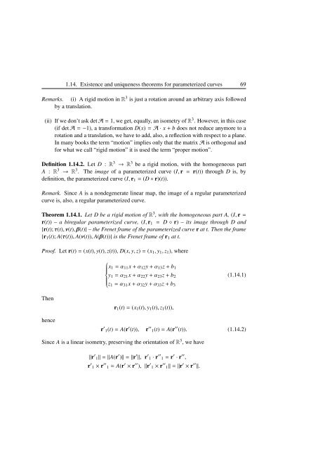
1.14. Existence and uniqueness theorems for parameterized curves 69
Remarks. (i) A rigid motion in R 3 is just a rotation around an arbitrary axis followed
by a translation.
(ii) If we don’t ask det A = 1, we get, equally, an isometry of R 3 . However, in this case
(if det A = −1), a transformation D(x) = A · x + b does not reduce anymore to a
rotation and a translation, we have to add, also, a reflection with respect to a plane.
In many books the term “motion” implies only that the matrix A is orthogonal and
for what we call “rigid motion” it is used the term “proper motion”.
Definition 1.14.2. Let D : R 3 → R 3 be a rigid motion, with the homogeneous part
A : R 3 → R 3 . The image of a parameterized curve (I, r = r(t)) through D is, by
definition, the parameterized curve (I, r1 = (D ◦ r)(t)).
Remark. Since A is a nondegenerate linear map, the image of a regular parameterized
curve is, also, a regular parameterized curve.
Theorem 1.14.1. Let D be a rigid motion of R 3 , with the homogeneous part A, (I, r =
r(t)) – a biregular parameterized curve, (I, r1 = D ◦ r) – its image through D and
{r(t); τ(t), ν(t), β(t)} – the Frenet frame of the parameterized curve r at t. Then the frame
{r1(t); A(τ(t)), A(ν(t)), A(β(t))} is the Frenet frame of r1 at t.
Proof. Let r(t) = (x(t), y(t), z(t)), D(x, y, z) = (x1, y1, z1), where
Then
hence
⎧
⎪⎨
⎪⎩
x1 = α11x + α12y + α13z + b1
y1 = α21x + α22y + α23z + b2
z1 = α31x + α32y + α33z + b3
r1(t) = (x1(t), y1(t), z1(t)),
(1.14.1)
r ′ 1(t) = A(r ′ (t)), r ′′ 1(t) = A(r ′′ (t)). (1.14.2)
Since A is a linear isometry, preserving the orientation of R 3 , we have
�r ′ 1� = �A(r ′ )� = �r ′ �, r ′ 1 · r ′′ 1 = r ′ · r ′′ ,
r ′ 1 × r ′′ 1 = A(r ′ × r ′′ ), �r ′ 1 × r ′′ 1� = �r ′ × r ′′ �.