- Page 1: Lectures on the Di
- Page 5 and 6: Contents Foreword 9 I Curves 11 1 S
- Page 7 and 8: Contents 7 4.5 The tangent vector s
- Page 9 and 10: Foreword This book is based on the
- Page 11: Part I Curves
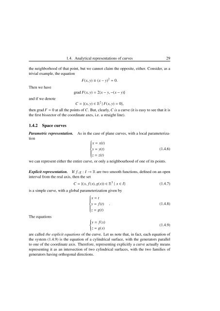
- Page 14 and 15: 14 Chapter 1. Space curves from the
- Page 16 and 17: 16 Chapter 1. Space curves Definiti
- Page 18 and 19: 18 Chapter 1. Space curves Figure 1
- Page 20 and 21: 20 Chapter 1. Space curves (I, r) i
- Page 22 and 23: 22 Chapter 1. Space curves Remark.
- Page 24 and 25: 24 Chapter 1. Space curves and ρ
- Page 26 and 27: 26 Chapter 1. Space curves given by
- Page 30 and 31: 30 Chapter 1. Space curves Implicit
- Page 32 and 33: 32 Chapter 1. Space curves Figure 1
- Page 34 and 35: 34 Chapter 1. Space curves Theorem
- Page 36 and 37: 36 Chapter 1. Space curves Explicit
- Page 38 and 39: 38 Chapter 1. Space curves From thi
- Page 40 and 41: 40 Chapter 1. Space curves Theorem
- Page 42 and 43: 42 Chapter 1. Space curves 1.7 The
- Page 44 and 45: 44 Chapter 1. Space curves Remark.
- Page 46 and 47: 46 Chapter 1. Space curves Figure 1
- Page 48 and 49: 48 Chapter 1. Space curves 1.9 Orie
- Page 50 and 51: 50 Chapter 1. Space curves 1.10 The
- Page 52 and 53: 52 Chapter 1. Space curves therefor
- Page 54 and 55: 54 Chapter 1. Space curves Proposit
- Page 56 and 57: 56 Chapter 1. Space curves or 1 + r
- Page 58 and 59: 58 Chapter 1. Space curves or c0 ·
- Page 60 and 61: 60 Chapter 1. Space curves Let ω b
- Page 62 and 63: 62 Chapter 1. Space curves Corollar
- Page 64 and 65: 64 Chapter 1. Space curves vector r
- Page 66 and 67: 66 Chapter 1. Space curves a) If a
- Page 68 and 69: 68 Chapter 1. Space curves d) We sh
- Page 70 and 71: 70 Chapter 1. Space curves Then: τ
- Page 72 and 73: 72 Chapter 1. Space curves 1.14.3 T
- Page 74 and 75: 74 Chapter 1. Space curves
- Page 76 and 77: 76 Chapter 2. Plane curves Proof. I
- Page 78 and 79:
78 Chapter 2. Plane curves By subst
- Page 80 and 81:
80 Chapter 2. Plane curves The foll
- Page 82 and 83:
82 Chapter 2. Plane curves c) J(Jv)
- Page 84 and 85:
84 Chapter 2. Plane curves therefor
- Page 86 and 87:
86 Chapter 2. Plane curves whence,
- Page 88 and 89:
88 Chapter 2. Plane curves Figure 2
- Page 90 and 91:
90 Chapter 2. Plane curves whence w
- Page 92 and 93:
92 Chapter 2. Plane curves where A(
- Page 94 and 95:
94 Chapter 2. Plane curves
- Page 96 and 97:
96 Chapter 3. The integration of th
- Page 98 and 99:
98 Chapter 3. The integration of th
- Page 100 and 101:
100 Chapter 3. The integration of t
- Page 102 and 103:
102 Chapter 3. The integration of t
- Page 104 and 105:
104 Problems 6. A straight line seg
- Page 106 and 107:
106 Problems 19. Show that the Bern
- Page 108 and 109:
108 Problems 35. Find the envelopes
- Page 110 and 111:
110 Problems d) x 2 y 2 = (a 2 −
- Page 112 and 113:
112 Chapter 3. The integration of t
- Page 115 and 116:
4.1 Parameterized surfaces (patches
- Page 117 and 118:
4.2. Surfaces 117 Explicit represen
- Page 119 and 120:
4.3. The equivalence of local param
- Page 121 and 122:
4.3. The equivalence of local param
- Page 123 and 124:
4.5. The tangent vector space, the
- Page 125 and 126:
4.5. The tangent vector space, the
- Page 127 and 128:
4.6. The orientation of surfaces 12
- Page 129 and 130:
and 4.6. The orientation of surface
- Page 131 and 132:
4.7. Differentiable maps on a surfa
- Page 133 and 134:
4.7. Differentiable maps on a surfa
- Page 135 and 136:
where 4.8. The differential of a sm
- Page 137 and 138:
4.9. The spherical map and the shap
- Page 139 and 140:
4.10. The first fundamental form of
- Page 141 and 142:
4.10. The first fundamental form of
- Page 143 and 144:
4.10. The first fundamental form of
- Page 145 and 146:
4.11. The matrix of the shape opera
- Page 147 and 148:
4.12. The second fundamental form o
- Page 149 and 150:
4.13. The normal curvature. The Meu
- Page 151 and 152:
4.14. Asymptotic directions and asy
- Page 153 and 154:
4.15. The classification of points
- Page 155 and 156:
4.15. The classification of points
- Page 157 and 158:
4.16. Principal directions and curv
- Page 159 and 160:
4.16. Principal directions and curv
- Page 161 and 162:
4.16. Principal directions and curv
- Page 163 and 164:
4.17. The fundamental equations of
- Page 165 and 166:
4.17. The fundamental equations of
- Page 167 and 168:
4.17. The fundamental equations of
- Page 169 and 170:
4.17. The fundamental equations of
- Page 171 and 172:
4.17. The fundamental equations of
- Page 173 and 174:
4.18. The Gauss’ egregium theorem
- Page 175 and 176:
4.19 Geodesics 4.19.1 Introduction
- Page 177 and 178:
4.19. Geodesics 177 will denote it
- Page 179 and 180:
4.19. Geodesics 179 where, as we kn
- Page 181 and 182:
Examples of geodesics 4.19. Geodesi
- Page 183 and 184:
4.19. Geodesics 183 Here, for the f
- Page 185 and 186:
5.1 Ruled surfaces CHAPTER 5 Specia
- Page 187 and 188:
5.1. Ruled surfaces 187 Figure 5.2:
- Page 189 and 190:
5.1. Ruled surfaces 189 Proof. Sinc
- Page 191 and 192:
5.1. Ruled surfaces 191 surfaces, g
- Page 193 and 194:
5.1. Ruled surfaces 193 The three c
- Page 195 and 196:
5.1. Ruled surfaces 195 We can rega
- Page 197 and 198:
5.1. Ruled surfaces 197 5.1.5 Devel
- Page 199 and 200:
5.1. Ruled surfaces 199 • The str
- Page 201 and 202:
5.2. Minimal surfaces 201 Given a c
- Page 203 and 204:
5.2. Minimal surfaces 203 The follo
- Page 205 and 206:
5.2. Minimal surfaces 205 Proof. Le
- Page 207 and 208:
5.2.3 Ruled minimal surfaces 5.2. M
- Page 209 and 210:
5.2. Minimal surfaces 209 asymptoti
- Page 211 and 212:
5.2. Minimal surfaces 211 as γ is
- Page 213 and 214:
5.3. Surfaces of constant curvature
- Page 215 and 216:
5.3. Surfaces of constant curvature
- Page 217 and 218:
1. We consider, in the coordinate p
- Page 219 and 220:
Problems 219 12. Show that the norm
- Page 221 and 222:
Problems 221 33. Find the envelope,
- Page 223 and 224:
Problems 223 45. Find the equation
- Page 225 and 226:
Problems 225 58. Find the second fu
- Page 227 and 228:
Problems 227 67. Through a point M
- Page 229 and 230:
[1] Bär, C. - Elementare Different
- Page 231 and 232:
Bibliography 231 [29] Jellet, J.H.
- Page 233 and 234:
affine normal, 109 arc length, 19,
- Page 235 and 236:
182, 185, 187-189, 202, 205, 213, 2
- Page 237:
torus, 118, 119, 154, 191, 217, 219


