Paramount GT-1100 Robotic Telescope Mount

Paramount User’s Guide page 49
6. Turn the Paramount ME Off, then On. The power on the Paramount ME must
be cycled before the new periodic error corrections take effect.
Note that the recording phase of the PEC training only records the error values. It does not
automatically transfer the recorded table to the flash or activate PEC adjustments.
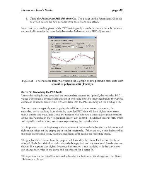
Figure 31 – The Periodic Error Correction tab's graph of raw periodic error data with
smoothed polynomial fit (TheSky).
Curve Fit: Smoothing the PEC Table
Unless the seeing is very good and the autoguiding settings are optimal, the recorded PEC
values will contain a considerable amount of noise and must be smoothed before the Upload
command is used to transfer the recorded table into the PEC memory on the TheSky TCS.
Because there are typically several pulleys in addition to the worm on the mount, the
smoothed curve resulting from the noisy recorded PEC data will have higher order terms
than a simple sine wave. The Curve-Fit function will compute a least squares polynomial fit
of the order entered in the “Polynomial order:” edit control. The default order is fifth, which
will typically result in a very nice curve representing the recorded data.
It is important that the beginning and end values of the recorded table (i.e. the left-most and
right-most values on the graph) are of similar magnitude. If they are not, it may indicate that
the polar alignment is poor, causing a significant drift during the recording phase.
The graphic above shows how the graphic will look after the Curve Fit function has been
selected. Both the original recorded data (the bumpy line) and the computed fitted curve are
shown. If it appears that higher frequency information is not modeled with the curve, you
can change the Order of the curve and experiment for a better fit.
The equation for the fitted line is also displayed at the bottom of the dialog once the Curve
Fit button is clicked.