TOOLED THICK COMPOSITES by ARVEN H. SAUNDERS III ...

Artificial neural networks have also been used to estimate reaction rate, as for example
by Lee and Rice (Lee, 1997). A neural net is “trained” by learning the input-output relationships
based on large amounts of known data. During training, the network adjusts its weights or
coefficients that link each neuron in the network, so that the output is correctly predicted from
the inputs. Backward propagation is a technique where errors in the input-output mapping are
fed backwards, from output to inputs, to correct the weights. The neural network model of Lee et
al predicts the reaction rate given the temperature and degree-of-cure inputs.
Other researchers have developed other useful model forms. Ng (Ng, 1999) developed
a 3rd order model that worked well with isothermal 8552 data. Shin et al (Shin, 2000) presented
a new technique for applying to an autocatalytic model that more accurately predicts the final
degree of cure. Costa et al (Costa, 2005) characterized carbon/epoxy 8552 using DSC and
rheometer data, as well as dynamic mechanical analysis (DMA) to develop cure kinetics (nth
order) and viscosity models
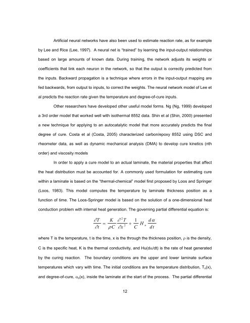
In order to apply a cure model to an actual laminate, the material properties that affect
the heat distribution must be accounted for. A commonly used formulation for estimating cure
within a laminate is based on the “thermal-chemical” model first proposed by Loos and Springer
(Loos, 1983). This model computes the temperature by laminate thickness position as a
function of time. The Loos-Springer model is based on the solution of a one-dimensional heat
conduction problem with internal heat generation. The governing partial differential equation is:
2
∂T
K ∂ T 1
= 2 +
∂t ρC
∂x
C
12
dα
H u
dt
where T is the temperature, t is the time, x is the through the thickness position, ρ is the density,
C is the specific heat, K is the thermal conductivity, and Hu(dα/dt) is the rate of heat generated
by the curing reaction. The boundary conditions are the upper and lower laminate surface
temperatures which vary with time. The initial conditions are the temperature distribution, To(x),
and degree-of-cure, αo(x), inside the laminate at the start of the process. The partial differential