nr. 477 - 2011 - Institut for Natur, Systemer og Modeller (NSM)

22 The DuCa Model
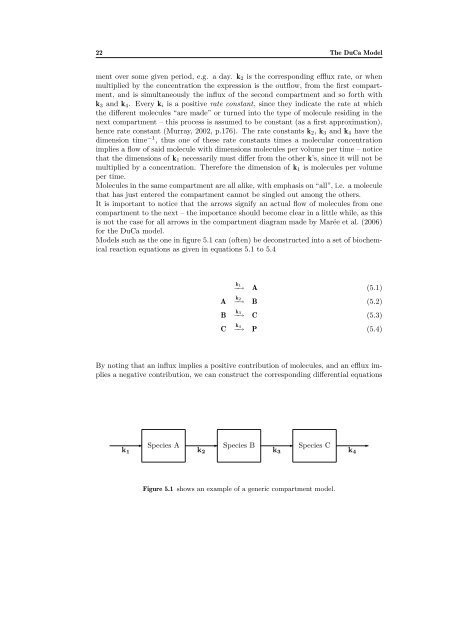
ment over some given period, e.g. a day. k2 is the corresponding efflux rate, or when
multiplied by the concentration the expression is the outflow, from the first compartment,
and is simultaneously the influx of the second compartment and so forth with
k3 and k4. Every ki is a positive rate constant, since they indicate the rate at which
the different molecules “are made” or turned into the type of molecule residing in the
next compartment – this process is assumed to be constant (as a first approximation),
hence rate constant (Murray, 2002, p.176). The rate constants k2, k3 and k4 have the
dimension time −1 , thus one of these rate constants times a molecular concentration
implies a flow of said molecule with dimensions molecules per volume per time – notice
that the dimensions of k1 necessarily must differ from the other k’s, since it will not be
multiplied by a concentration. Therefore the dimension of k1 is molecules per volume
per time.
Molecules in the same compartment are all alike, with emphasis on “all”, i.e. a molecule
that has just entered the compartment cannot be singled out among the others.
It is important to notice that the arrows signify an actual flow of molecules from one
compartment to the next – the importance should become clear in a little while, as this
is not the case for all arrows in the compartment diagram made by Marée et al. (2006)
for the DuCa model.
Models such as the one in figure 5.1 can (often) be deconstructed into a set of biochemical
reaction equations as given in equations 5.1 to 5.4
k1
−→ A (5.1)
A k2
−→ B (5.2)
B k3
−→ C (5.3)
C k4
−→ P (5.4)
By noting that an influx implies a positive contribution of molecules, and an efflux implies
a negative contribution, we can construct the corresponding differential equations
k1
✲
Species A
k2
✲
Species B
k3
✲
Species C
Figure 5.1 shows an example of a generic compartment model.
k4
✲