nr. 477 - 2011 - Institut for Natur, Systemer og Modeller (NSM)

More documents

Recommendations

Info

66 A Brief Introduction to Bifurcation Analysis and Numerical Methods to induce a bifurcation, we speak of a codimension two bifurcation, and so forth up to n parameters. An instructive one-dimensional example is: ˙x = r + x 2 (7.1) For r < 0 there are two fixed points (x ∗ = ± √ r). One is stable and one is unstable, as one can see by plotting ˙x in a ˙xx-coordinate system. For r → 0 the two fixed points will approach each other. Finally at r = 0 they will coalesce to become a half-stable point or a saddle-point, i.e. a point that is attracting from one side and repelling from the other – the flow is in one direction. Immediately after r becomes positive the fixed points (on the real line) no longer exist. They have annihilated; a bifurcation has occurred. r ∗ = 0 is called the bifurcation point or bifurcation value, and r is in this case called the bifurcation parameter. More specifically the bifurcation value is defined as a value r ∗ for which the flow of the system in equation 7.1 is not structurally stable (Guckenheimer and Holmes, 2002, p.119). This was an example of a so-called saddle-node bifurcation, which is one of the generic or archetypical local bifurcations. The other generic one-dimensional bifurcations are (Guckenheimer and Holmes, 2002, p.145-148) The transcritical bifurcation this one arises from the system ˙x = rx − x 2 . When r is negative there are two fixed points – one stable (at the origin) and one unstable (at r). For r = 0 there is only one half-stable fixed point (at the origin), and for r > 0 there is once again two fixed points, but now the the fixed point at the origin is unstable, while x ∗ = r is stable – an exchange of stability has occurred. The pitchfork bifurcation this one comes in two categories, a subcritical (arises from ˙x = rx + x 3 ), and a supercritical (arises from ˙x = rx − x 3 ). These two are qualitatively different, but what they have in common is that one fixed point branches into three fixed points as r crosses 0. There is one additional bifurcation that can be categorized as generic, namely the Andronov-Hopf bifurcation or more commonly simply the Hopf bifurcation. This bifurcation type merits a little more explanation, so we have endowed it with its own section. Introducing the Hopf bifurcation also allows us to give a brief description of how some of the more interesting behaviors a system can exhibit come about, i.e. why complex eigenvalues entail spirals or closed orbits. 7.2 The Hopf bifurcation The Hopf bifurcation differs from the other bifurcations in that it cannot occur in onedimensional systems, so let us start by supposing that we have a system of autonomous nonlinear differential equations that depend on a bifurcation parameter r ∈ R, and that we have linearized the system around a fixed point, i.e. we have disposed of the higher order nonlinear terms. The linear system can be written in the from ˙x = Ax (7.2) with initial condition x(0) = x0, and A is the Jacobian. Now suppose that we find the corresponding characteristic polynomial from which we obtain the eigenvalues. Then
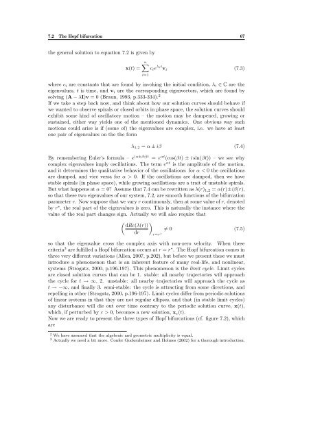
7.2 The Hopf bifurcation 67 the general solution to equation 7.2 is given by x(t) = n i=1 cie λit vi (7.3) where ci are constants that are found by invoking the initial condition, λi ∈ C are the eigenvalues, t is time, and vi are the corresponding eigenvectors, which are found by solving (A − λI)v = 0 (Braun, 1993, p.333-334). 2 If we take a step back now, and think about how our solution curves should behave if we wanted to observe spirals or closed orbits in phase space, the solution curves should exhibit some kind of oscillatory motion – the motion may be dampened, growing or sustained, either way yields one of the mentioned dynamics. One obvious way such motions could arise is if (some of) the eigenvalues are complex, i.e. we have at least one pair of eigenvalues on the the form λ1,2 = α ± iβ (7.4) By remembering Euler’s formula – e (α±βi)t = eαt (cos(βt) ± i sin(βt)) – we see why complex eigenvalues imply oscillations. The term eαt is the amplitude of the motion, and it determines the qualitative behavior of the oscillations: for α < 0 the oscillations are damped, and vice versa for α > 0. If the oscillations are damped, then we have stable spirals (in phase space), while growing oscillations are a trait of unstable spirals. But what happens at α = 0? Assume that 7.4 can be rewritten as λ(r)1,2 = α(r)±iβ(r), so that these two eigenvalues of our system, 7.2, are smooth functions of the bifurcation parameter r. Now suppose that we vary r continuously, then at some value of r, denoted by r∗ , the real part of the eigenvalues is zero. This is naturally the instance where the value of the real part changes sign. Actually we will also require that dRe(λ(r)) = 0 (7.5) dr so that the eigenvalue cross the complex axis with non-zero velocity. When these criteria 3 are fulfilled a Hopf bifurcation occurs at r = r ∗ . The Hopf bifurcation comes in three very different variations (Allen, 2007, p.202), but before we present these we must introduce a phenomenon that is an inherent feature of many real-life, and nonlinear, systems (Strogatz, 2000, p.196-197). This phenomenon is the limit cycle. Limit cycles are closed solution curves that can be 1. stable: all nearby trajectories will approach the cycle for t → ∞, 2. unstable: all nearby trajectories will approach the cycle as t → −∞, and finally 3. semi-stable: the cycle is attracting from some directions, and repelling in other (Strogatz, 2000, p.196-197). Limit cycles differ from periodic solutions of linear systems in that they are not regular ellipses, and that (in stable limit cycles) any disturbance will die out over time contrary to the periodic solution curve, x(t), which, if perturbed by ε > 0, becomes a new solution, xε(t). Now we are ready to present the three types of Hopf bifurcations (cf. figure 7.2), which are 2 We have assumed that the algebraic and geometric multiplicity is equal. 3 Actually we need a bit more. Confer Guckenheimer and Holmes (2002) for a thorough introduction. r=r ∗
Page 1 and 2:
- I, OM OG MED MATEMATIK OG FYSIK E
Page 3 and 4:
Exploring Treatment Strategies for
Page 5:
Preface iii questions that were out
Page 8 and 9:
vi Contents Significance of the Apo
Page 10 and 11:
List of Tables 5.1 summarizes the m
Page 12 and 13:
x List of Figures 8.3 Phase space p
Page 14 and 15:
xii
Page 16 and 17:
2 Introduction In the following dec
Page 18 and 19:
4 Introduction There are several sc
Page 20 and 21:
6 Introduction because I had to mak
Page 22 and 23:
8 Type 1 Diabetes and Its Etiology
Page 24 and 25:
10 Type 1 Diabetes and Its Etiology
Page 27 and 28:
3 Prospects for Therapy - A Mini Re
Page 29 and 30: 3.3 Gastrin 15 eration in situ Urus
Page 31 and 32: 4 Mathematical Modelling The langua
Page 33 and 34: 5 The DuCa Model In the following w
Page 35 and 36: 5.3 The DuCa Model - An Appetiser 2
Page 37 and 38: 5.4 The DuCa Model - Compartment Mo
Page 43 and 44: 5.6 Our Compartment Model 29 migrat
Page 45 and 46: 5.6 Our Compartment Model 31 a ✓
Page 47 and 48: 5.7 Discussion of Marée et al. (20
Page 49 and 50: 5.7 Discussion of Marée et al. (20
Page 51 and 52: 5.8 Discussion of Parameters 37 Fig
Page 53 and 54: 5.8 Discussion of Parameters 39 Par
Page 55 and 56: 5.8 Discussion of Parameters 41 tha
Page 57: 5.8 Discussion of Parameters 43 Fig
Page 60 and 61: 46 The Intermediated Model The diff
Page 62 and 63: 48 The Intermediated Model expected
Page 64 and 65: 50 The Intermediated Model Stabilit
Page 66 and 67: 52 The Intermediated Model restrict
Page 68 and 69: 54 The Intermediated Model We see t
Page 70 and 71: 56 The Intermediated Model paramete
Page 72 and 73: 58 The Intermediated Model ✻ Ma(t
Page 74 and 75: 60 The Intermediated Model 6.2 The
Page 76 and 77: 62 The Intermediated Model ✻ Ma(t
Page 79: 7 A Brief Introduction to Bifurcati
Page 83 and 84: 7.3 Biological Relevance of Bifurca
Page 85: 7.5 Locating the Fixed Points 71 Ev
Page 88 and 89: 74 Bifurcation Diagrams and Analysi
Page 112 and 113: 98 Discussion of the Bifurcation An
Page 114 and 115: 100 Discussion of the Bifurcation A
Page 116 and 117: 102
Page 118 and 119: 104
Page 120 and 121: 106 Expanding and Modifying the DuC
Page 130 and 131:
116 Expanding and Modifying the DuC
Page 132 and 133:
118 Discussion of the Expanded Mode
Page 134 and 135:
120 Discussion of the Expanded Mode
Page 136 and 137:
122
Page 138 and 139:
124
Page 140 and 141:
126 Bibliography Christen, U. and M
Page 142 and 143:
128 Bibliography Notkins, A. L. and
Page 144 and 145:
130 Bibliography Yu, J. and G. S. E
Page 146 and 147:
132 Mathematical Appendices the com
Page 148 and 149:
134 Mathematical Appendices in that
Page 150 and 151:
136 Mathematical Appendices A.6 Dim
Page 152 and 153:
138
Page 154 and 155:
140 Additional Figures Figure B.2 P
Page 156 and 157:
142 Additional Figures B.2 Eigenval
Page 158 and 159:
144 Additional Figures Figure B.8 P
Page 160 and 161:
Page 162 and 163:
148 Additional Figures Figure B.14
Page 164 and 165:
Page 166 and 167:
Page 168 and 169:
Page 170 and 171:
Page 172 and 173:
158 matlab Code w(r+1)=w(r)+dw; g=w
Page 174 and 175:
160 matlab Code end V_11(r)=E(1); V
Page 176 and 177:
162 matlab Code n=675; w_5=0; dw_5=
Page 178 and 179:
164 matlab Code M=M’; % end s_7(r
Page 180 and 181:
166 matlab Code w_7,V_34,’.b’,w
Page 182 and 183:
168 matlab Code M=M’; % M must be
Page 184 and 185:
170 matlab Code %options = odeset(
Page 186 and 187:
172
Page 188 and 189:
174 Index value, 73 Bifurcation Ana
Page 190 and 191:
176 Index of diabetes, 2 Michaelis
show all

nr. 477 - 2011 - Institut for Natur, Systemer og Modeller (NSM)

You also want an ePaper? Increase the reach of your titles

Delete template?

Save as template?