nr. 477 - 2011 - Institut for Natur, Systemer og Modeller (NSM)

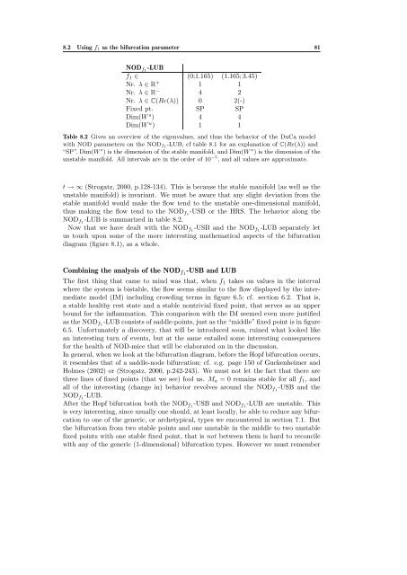
8.2 Using f1 as the bifurcation parameter 81
NODf1-LUB
f1 ∈ (0;1.165) (1.165; 3.45)
Nr. λ ∈ R + 1 1
Nr. λ ∈ R − 4 2
Nr. λ ∈ C(Re(λ)) 0 2(-)
Fixed pt. SP SP
Dim(W s ) 4 4
Dim(W u ) 1 1
Table 8.2 Gives an overview of the eigenvalues, and thus the behavior of the DuCa model
with NOD parameters on the NODf1-LUB; cf table 8.1 for an explanation of C(Re(λ)) and
“SP”. Dim(W s ) is the dimension of the stable manifold, and Dim(W u ) is the dimension of the
unstable manifold. All intervals are in the order of 10 −5 , and all values are approximate.
t → ∞ (Strogatz, 2000, p.128-134). This is because the stable manifold (as well as the
unstable manifold) is invariant. We must be aware that any slight deviation from the
stable manifold would make the flow tend to the unstable one-dimensional manifold,
thus making the flow tend to the NODf1-USB or the HRS. The behavior along the
NODf1-LUB is summarized in table 8.2.
Now that we have dealt with the NODf1-USB and the NODf1-LUB separately let
us touch upon some of the more interesting mathematical aspects of the bifurcation
diagram (figure 8.1), as a whole.
Combining the analysis of the NODf1-USB and LUB
The first thing that came to mind was that, when f1 takes on values in the interval
where the system is bistable, the flow seems similar to the flow displayed by the intermediate
model (IM) including crowding terms in figure 6.5; cf. section 6.2. That is,
a stable healthy rest state and a stable nontrivial fixed point, that serves as an upper
bound for the inflammation. This comparison with the IM seemed even more justified
as the NODf1-LUB consists of saddle-points, just as the “middle” fixed point is in figure
6.5. Unfortunately a discovery, that will be introduced soon, ruined what looked like
an interesting turn of events, but at the same entailed some interesting consequences
for the health of NOD-mice that will be elaborated on in the discussion.
In general, when we look at the bifurcation diagram, before the Hopf bifurcation occurs,
it resembles that of a saddle-node bifurcation; cf. e.g. page 150 of Guckenheimer and
Holmes (2002) or (Strogatz, 2000, p.242-243). We must not let the fact that there are
three lines of fixed points (that we see) fool us. Ma = 0 remains stable for all f1, and
all of the interesting (change in) behavior revolves around the NODf1-USB and the
NODf1-LUB.
After the Hopf bifurcation both the NODf1-USB and NODf1-LUB are unstable. This
is very interesting, since usually one should, at least locally, be able to reduce any bifurcation
to one of the generic, or archetypical, types we encountered in section 7.1. But
the bifurcation from two stable points and one unstable in the middle to two unstable
fixed points with one stable fixed point, that is not between them is hard to reconcile
with any of the generic (1-dimensional) bifurcation types. However we must remember