nr. 477 - 2011 - Institut for Natur, Systemer og Modeller (NSM)

76 Bifurcation Diagrams and Analysis
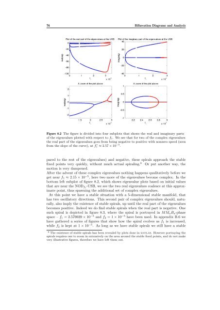
Figure 8.2 The figure is divided into four subplots that shows the real and imaginary parts
of the eigenvalues plotted with respect to f1. We see that for two of the complex eigenvalues
the real part of the eigenvalues goes from being negative to positive with nonzero speed (seen
from the slope of the curve), at f ∗ 1 ≈ 2.57 × 10 −5 .
pared to the rest of the eigenvalues) and negative, these spirals approach the stable
fixed points very quickly, without much actual spiraling. 6 Or put another way, the
motion is very dampened.
After the advent of these complex eigenvalues nothing happens qualitatively before we
get near f1 ≈ 2.15 × 10 −5 , here two more of the eigenvalues become complex. In the
bottom left subplot of figure 8.2, which shows eigenvalue plots based on initial values
that are near the NODf1-USB, we see the two real eigenvalues coalesce at this approx-
imate point, thus spawning the additional set of complex eigenvalues.
At this point we have a stable situation with a 5-dimensional stable manifold, that
has two oscillatory directions. This second pair of complex eigenvalues should, naturally,
also imply the existence of stable spirals, up until the real part of the eigenvalues
becomes positive. Indeed we do find stable spirals when the real part is negative. One
such spiral is depicted in figure 8.3, where the spiral is portrayed in MMaBa-phase
space – f1 = 2.570039 × 10 −5 and f2 = 1 × 10 −5 have been used. In appendix B.6 we
have gathered a series of figures that show how the spiral evolves as f1 is increased,
while f2 is kept at 1 × 10 −5 . As long as we have stable spirals we still have a stable
6 The existence of stable spirals has been revealed by plots done in matlab. However portraying the
spirals requires one to zoom in extensively on the area around the stable fixed points, and do not make
very illustrative figures, therefore we have left them out.