Edge-connectivity of undirected and directed hypergraphs
Edge-connectivity of undirected and directed hypergraphs
Edge-connectivity of undirected and directed hypergraphs

You also want an ePaper? Increase the reach of your titles
YUMPU automatically turns print PDFs into web optimized ePapers that Google loves.
Section 6.4. Directed network design problems with orientation constraints 107<br />
v1<br />
a1<br />
v2<br />
v4<br />
A1<br />
a2<br />
v3<br />
v5<br />
v6<br />
A2<br />
ϕ(v5)<br />
ϕ(v1)<br />
ϕ({v2, v4})<br />
w1<br />
ϕ(v3)<br />
ϕ(v6)<br />
Figure 6.3: Construction <strong>of</strong> the network matrix in Theorem 6.14<br />
positive on two intersecting sets X <strong>and</strong> Y where p(X), p(Y ) > 0; let α = min{p(X), p(Y )}.<br />
Decrease y ∗ (X) <strong>and</strong> y ∗ (Y ) by α, <strong>and</strong> increase y ∗ (X ∩ Y ) <strong>and</strong> y ∗ (X ∪ Y ) by α. Since<br />
ϱa(X) + ϱa(Y ) ≥ ϱa(X ∩ Y ) + ϱa(X ∪ Y ) for each hyperarc a, the inequality (6.11) is<br />
preserved. The positively intersecting supermodularity <strong>of</strong> p implies that the dual objective<br />
function (6.12) does not decrease. By Claim 2.5, after a finite number <strong>of</strong> uncrossing steps,<br />
we obtain an optimal dual solution where y ∗ is positive on a laminar family F.<br />
Modify the system (S) by replacing (6.8) with<br />
ϱx(Z) ≥ p(Z) for every Z ∈ F; (6.13)<br />
let us denote this system by (S ′ ). Then (y ∗ , z ∗ ) remains a feasible dual solution, <strong>and</strong> it is<br />
obviously optimal. Thus if the modified system has an integral optimal dual solution, it<br />
is optimal for the dual <strong>of</strong> (S) as well. The rest <strong>of</strong> the pro<strong>of</strong> consists <strong>of</strong> showing that the<br />
system (S ′ ) can be described by a network matrix, hence it has an integral dual optimal<br />
solution by Proposition 2.25.<br />
The construction <strong>of</strong> the corresponding network is shown on Figure 6.3. The rows <strong>of</strong><br />
the network matrix will correspond to the edges <strong>of</strong> a <strong>directed</strong> tree T ′ = (W ′ , A ′ 1), <strong>and</strong> the<br />
corresponding lower <strong>and</strong> upper bounds will be denoted by l ′ <strong>and</strong> u ′ . The laminar family F<br />
has a tree-representation (T, ϕ) where T = (W, A1) is an arborescence; T ′ will include T as<br />
a subtree. For an edge e ∈ A1 let l ′ (e) = −∞ <strong>and</strong> u ′ (e) = −p(ϕ −1 (We)), where We is the<br />
component <strong>of</strong> T − e entered by e. The node set W ′ is obtained by adding new nodes wi<br />
(i = 1, . . . , t) to W (that is, one new node wi for each orientation constraint set Ai which<br />
consists <strong>of</strong> semi-parallel hyperedges). For a set Z ⊆ V let wZ ∈ W denote the root node <strong>of</strong><br />
the minimal subtree <strong>of</strong> T containing all nodes <strong>of</strong> ϕ(Z). To finish the construction <strong>of</strong> T ′ , add<br />
an edge ei = wZi wi to A ′ 1 for i = 1, . . . , t, where Zi is the node set <strong>of</strong> the hyperedge whose<br />
orientations are in Ai. Define the corresponding lower <strong>and</strong> upper bounds as l ′ (ei) = li,<br />
u ′ (ei) = ui.<br />
w2