CHAPTER 13 Simple Linear Regression
CHAPTER 13 Simple Linear Regression
CHAPTER 13 Simple Linear Regression

You also want an ePaper? Increase the reach of your titles
YUMPU automatically turns print PDFs into web optimized ePapers that Google loves.
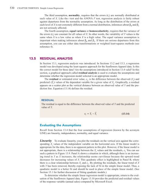
530 <strong>CHAPTER</strong> THIRTEEN <strong>Simple</strong> <strong>Linear</strong> <strong>Regression</strong><br />
The third assumption, normality, requires that the errors (ε i<br />
) are normally distributed at<br />
each value of X. Like the t test and the ANOVA F test, regression analysis is fairly robust<br />
against departures from the normality assumption. As long as the distribution of the errors at<br />
each level of X is not extremely different from a normal distribution, inferences about β 0<br />
and β 1<br />
are not seriously affected.<br />
The fourth assumption, equal variance or homoscedasticity, requires that the variance of<br />
the errors (ε i<br />
) are constant for all values of X. In other words, the variability of Y values is the<br />
same when X is a low value as when X is a high value. The equal variance assumption is<br />
important when making inferences about β 0<br />
and β 1<br />
. If there are serious departures from this<br />
assumption, you can use either data transformations or weighted least-squares methods (see<br />
reference 4).<br />
<strong>13</strong>.5 RESIDUAL ANALYSIS<br />
In Section <strong>13</strong>.1, regression analysis was introduced. In Sections <strong>13</strong>.2 and <strong>13</strong>.3, a regression<br />
model was developed using the least-squares approach for the Sunflowers Apparel data. Is this<br />
the correct model for these data? Are the assumptions introduced in Section <strong>13</strong>.4 valid? In this<br />
section, a graphical approach called residual analysis is used to evaluate the assumptions and<br />
determine whether the regression model selected is an appropriate model.<br />
The residual or estimated error value, e i<br />
, is the difference between the observed (Y i<br />
) and<br />
predicted ( Yˆ i ) values of the dependent variable for a given value of X i<br />
. Graphically, a residual<br />
appears on a scatter plot as the vertical distance between an observed value of Y and the prediction<br />
line. Equation (<strong>13</strong>.14) defines the residual.<br />
RESIDUAL<br />
The residual is equal to the difference between the observed value of Y and the predicted<br />
value of Y.<br />
ei = Yi −Yˆ<br />
i<br />
(<strong>13</strong>.14)<br />
Evaluating the Assumptions<br />
Recall from Section <strong>13</strong>.4 that the four assumptions of regression (known by the acronym<br />
LINE) are linearity, independence, normality, and equal variance.<br />
<strong>Linear</strong>ity To evaluate linearity, you plot the residuals on the vertical axis against the corresponding<br />
X i<br />
values of the independent variable on the horizontal axis. If the linear model is<br />
appropriate for the data, there is no apparent pattern in this plot. However, if the linear model is<br />
not appropriate, there is a relationship between the X i<br />
values and the residuals, e i<br />
. You can see<br />
such a pattern in Figure <strong>13</strong>.9. Panel A shows a situation in which, although there is an increasing<br />
trend in Y as X increases, the relationship seems curvilinear because the upward trend<br />
decreases for increasing values of X. This quadratic effect is highlighted in Panel B, where<br />
there is a clear relationship between X i<br />
and e i<br />
. By plotting the residuals, the linear trend of X<br />
with Y has been removed, thereby exposing the lack of fit in the simple linear model. Thus, a<br />
quadratic model is a better fit and should be used in place of the simple linear model. (See<br />
Section 15.1 for further discussion of fitting quadratic models.)<br />
To determine whether the simple linear regression model is appropriate, return to the evaluation<br />
of the Sunflowers Apparel data. Figure <strong>13</strong>.10 provides the predicted and residual values<br />
of the response variable (annual sales) computed by Microsoft Excel.