CHAPTER 13 Simple Linear Regression
CHAPTER 13 Simple Linear Regression
CHAPTER 13 Simple Linear Regression

You also want an ePaper? Increase the reach of your titles
YUMPU automatically turns print PDFs into web optimized ePapers that Google loves.
518 <strong>CHAPTER</strong> THIRTEEN <strong>Simple</strong> <strong>Linear</strong> <strong>Regression</strong><br />
VISUAL EXPLORATIONS Exploring <strong>Simple</strong> <strong>Linear</strong> <strong>Regression</strong> Coefficients<br />
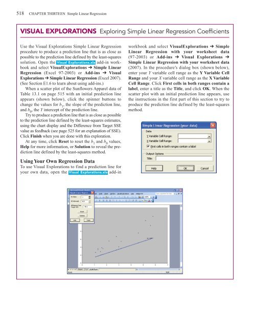
Use the Visual Explorations <strong>Simple</strong> <strong>Linear</strong> <strong>Regression</strong><br />
procedure to produce a prediction line that is as close as<br />
possible to the prediction line defined by the least-squares<br />
solution. Open the Visual Explorations.xla add-in workbook<br />
and select VisualExplorations ➔ <strong>Simple</strong> <strong>Linear</strong><br />
<strong>Regression</strong> (Excel 97-2003) or Add-ins ➔ Visual<br />
Explorations ➔ <strong>Simple</strong> <strong>Linear</strong> <strong>Regression</strong> (Excel 2007).<br />
(See Section E1.6 to learn about using add-ins.)<br />
When a scatter plot of the Sunflowers Apparel data of<br />
Table <strong>13</strong>.1 on page 515 with an initial prediction line<br />
appears (shown below), click the spinner buttons to<br />
change the values for b 1<br />
, the slope of the prediction line,<br />
and b 0<br />
, the Y intercept of the prediction line.<br />
Try to produce a prediction line that is as close as possible<br />
to the prediction line defined by the least-squares estimates,<br />
using the chart display and the Difference from Target SSE<br />
value as feedback (see page 525 for an explanation of SSE).<br />
Click Finish when you are done with this exploration.<br />
At any time, click Reset to reset the b 1<br />
and b 0<br />
values,<br />
Help for more information, or Solution to reveal the prediction<br />
line defined by the least-squares method.<br />
workbook and select VisualExplorations ➔ <strong>Simple</strong><br />
<strong>Linear</strong> <strong>Regression</strong> with your worksheet data<br />
(97-2003) or Add-ins ➔ Visual Explorations ➔<br />
<strong>Simple</strong> <strong>Linear</strong> <strong>Regression</strong> with your worksheet data<br />
(2007). In the procedure’s dialog box (shown below),<br />
enter your Y variable cell range as the Y Variable Cell<br />
Range and your X variable cell range as the X Variable<br />
Cell Range. Click First cells in both ranges contain a<br />
label, enter a title as the Title, and click OK. When the<br />
scatter plot with an initial prediction line appears, use<br />
the instructions in the first part of this section to try to<br />
produce the prediction line defined by the least-squares<br />
method.<br />
Using Your Own <strong>Regression</strong> Data<br />
To use Visual Explorations to find a prediction line for<br />
your own data, open the Visual Explorations.xla add-in