CHAPTER 13 Simple Linear Regression

538 CHAPTER THIRTEEN Simple Linear Regression
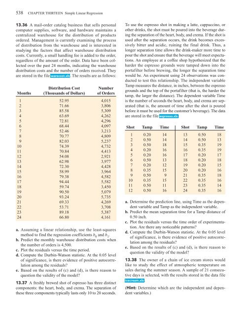
13.36 A mail-order catalog business that sells personal
computer supplies, software, and hardware maintains a
centralized warehouse for the distribution of products
ordered. Management is currently examining the process
of distribution from the warehouse and is interested in
studying the factors that affect warehouse distribution
costs. Currently, a small handling fee is added to the order,
regardless of the amount of the order. Data have been collected
over the past 24 months, indicating the warehouse
distribution costs and the number of orders received. They
are stored in the file warecost.xls. The results are as follows:
Distribution Cost Number
Months (Thousands of Dollars) of Orders
1 52.95 4,015
2 71.66 3,806
3 85.58 5,309
4 63.69 4,262
5 72.81 4,296
6 68.44 4,097
7 52.46 3,213
8 70.77 4,809
9 82.03 5,237
10 74.39 4,732
11 70.84 4,413
12 54.08 2,921
13 62.98 3,977
14 72.30 4,428
15 58.99 3,964
16 79.38 4,582
17 94.44 5,582
18 59.74 3,450
19 90.50 5,079
20 93.24 5,735
21 69.33 4,269
22 53.71 3,708
23 89.18 5,387
24 66.80 4,161
a. Assuming a linear relationship, use the least-squares
method to find the regression coefficients b 0
and b 1
.
b. Predict the monthly warehouse distribution costs when
the number of orders is 4,500.
c. Plot the residuals versus the time period.
d. Compute the Durbin-Watson statistic. At the 0.05 level
of significance, is there evidence of positive autocorrelation
among the residuals?
e. Based on the results of (c) and (d), is there reason to
question the validity of the model?
13.37 A freshly brewed shot of espresso has three distinct
components: the heart, body, and crema. The separation of
these three components typically lasts only 10 to 20 seconds.
To use the espresso shot in making a latte, cappuccino, or
other drinks, the shot must be poured into the beverage during
the separation of the heart, body, and crema. If the shot is
used after the separation occurs, the drink becomes excessively
bitter and acidic, ruining the final drink. Thus, a
longer separation time allows the drink-maker more time to
pour the shot and ensure that the beverage will meet expectations.
An employee at a coffee shop hypothesized that the
harder the espresso grounds were tamped down into the
portafilter before brewing, the longer the separation time
would be. An experiment using 24 observations was conducted
to test this relationship. The independent variable
Tamp measures the distance, in inches, between the espresso
grounds and the top of the portafilter (that is, the harder the
tamp, the larger the distance). The dependent variable Time
is the number of seconds the heart, body, and crema are separated
(that is, the amount of time after the shot is poured
before it must be used for the customer’s beverage). The data
are stored in the file espresso.xls:
Shot Tamp Time Shot Tamp Time
1 0.20 14 13 0.50 18
2 0.50 14 14 0.50 13
3 0.50 18 15 0.35 19
4 0.20 16 16 0.35 19
5 0.20 16 17 0.20 17
6 0.50 13 18 0.20 18
7 0.20 12 19 0.20 15
8 0.35 15 20 0.20 16
9 0.50 9 21 0.35 18
10 0.35 15 22 0.35 16
11 0.50 11 23 0.35 14
12 0.50 16 24 0.35 16
a. Determine the prediction line, using Time as the dependent
variable and Tamp as the independent variable.
b. Predict the mean separation time for a Tamp distance of
0.50 inch.
c. Plot the residuals versus the time order of experimentation.
Are there any noticeable patterns?
d. Compute the Durbin-Watson statistic. At the 0.05 level
of significance, is there evidence of positive autocorrelation
among the residuals?
e. Based on the results of (c) and (d), is there reason to
question the validity of the model?
13.38 The owner of a chain of ice cream stores would
like to study the effect of atmospheric temperature on
sales during the summer season. A sample of 21 consecutive
days is selected, with the results stored in the data file
icecream.xls.
(Hint: Determine which are the independent and dependent
variables.)