CHAPTER 13 Simple Linear Regression

532 CHAPTER THIRTEEN Simple Linear Regression
Independence You can evaluate the assumption of independence of the errors by plotting
the residuals in the order or sequence in which the data were collected. Data collected over
periods of time sometimes exhibit an autocorrelation effect among successive observations. In
these instances, there is a relationship between consecutive residuals. If this relationship exists
(which violates the assumption of independence), it is apparent in the plot of the residuals versus
the time in which the data were collected. You can also test for autocorrelation by using the
Durbin-Watson statistic, which is the subject of Section 13.6. Because the Sunflowers Apparel
data were collected during the same time period, you do not need to evaluate the independence
assumption.
Normality You can evaluate the assumption of normality in the errors by tallying the residuals
into a frequency distribution and displaying the results in a histogram (see Section 2.3).
For the Sunflowers Apparel data, the residuals have been tallied into a frequency distribution in
Table 13.3. (There are an insufficient number of values, however, to construct a histogram.)
You can also evaluate the normality assumption by comparing the actual versus theoretical values
of the residuals or by constructing a normal probability plot of the residuals (see Section
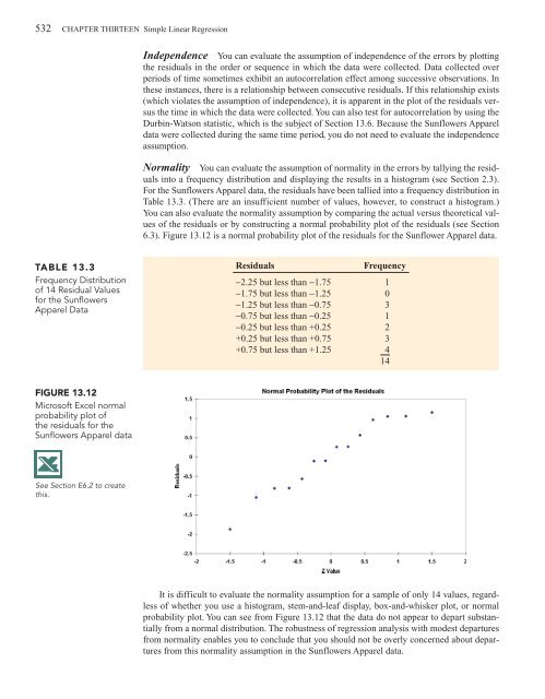
6.3). Figure 13.12 is a normal probability plot of the residuals for the Sunflower Apparel data.
TABLE 13.3
Frequency Distribution
of 14 Residual Values
for the Sunflowers
Apparel Data
Residuals
Frequency
−2.25 but less than −1.75 1
−1.75 but less than −1.25 0
−1.25 but less than −0.75 3
−0.75 but less than −0.25 1
−0.25 but less than +0.25 2
+0.25 but less than +0.75 3
+0.75 but less than +1.25 4
14
FIGURE 13.12
Microsoft Excel normal
probability plot of
the residuals for the
Sunflowers Apparel data
See Section E6.2 to create
this.
It is difficult to evaluate the normality assumption for a sample of only 14 values, regardless
of whether you use a histogram, stem-and-leaf display, box-and-whisker plot, or normal
probability plot. You can see from Figure 13.12 that the data do not appear to depart substantially
from a normal distribution. The robustness of regression analysis with modest departures
from normality enables you to conclude that you should not be overly concerned about departures
from this normality assumption in the Sunflowers Apparel data.