sparse grid method in the libor market model. option valuation and the
sparse grid method in the libor market model. option valuation and the
sparse grid method in the libor market model. option valuation and the
Create successful ePaper yourself
Turn your PDF publications into a flip-book with our unique Google optimized e-Paper software.
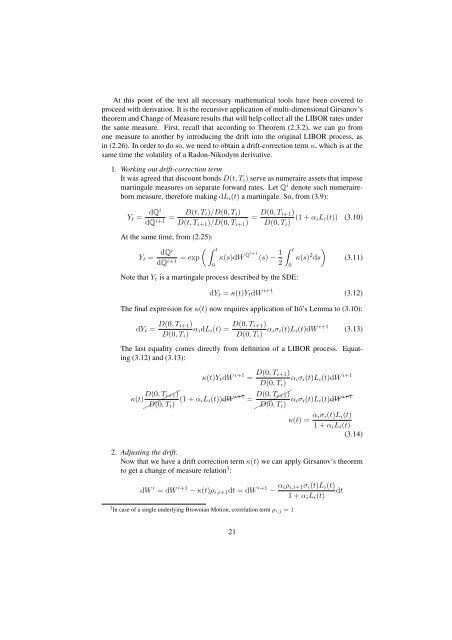
At this po<strong>in</strong>t of <strong>the</strong> text all necessary ma<strong>the</strong>matical tools have been covered to<br />
proceed with derivation. It is <strong>the</strong> recursive application of multi-dimensional Girsanov’s<br />
<strong>the</strong>orem <strong>and</strong> Change of Measure results that will help collect all <strong>the</strong> LIBOR rates under<br />
<strong>the</strong> same measure. First, recall that accord<strong>in</strong>g to Theorem (2.3.2), we can go from<br />
one measure to ano<strong>the</strong>r by <strong>in</strong>troduc<strong>in</strong>g <strong>the</strong> drift <strong>in</strong>to <strong>the</strong> orig<strong>in</strong>al LIBOR process, as<br />
<strong>in</strong> (2.26). In order to do so, we need to obta<strong>in</strong> a drift-correction term κ, which is at <strong>the</strong><br />
same time <strong>the</strong> volatility of a Radon-Nikodym derivative.<br />
1. Work<strong>in</strong>g out drift-correction term<br />
It was agreed that discount bonds D(t, T i ) serve as numeraire assets that impose<br />
mart<strong>in</strong>gale measures on separate forward rates. Let Q i denote such numeraireborn<br />
measure, <strong>the</strong>refore mak<strong>in</strong>g dL i (t) a mart<strong>in</strong>gale. So, from (3.9):<br />
Y t =<br />
dQi<br />
dQ i+1 = D(t, T i)/D(0, T i )<br />
D(t, T i+1 )/D(0, T i+1 ) = D(0, T i+1)<br />
D(0, T i ) (1 + α iL i (t)) (3.10)<br />
At <strong>the</strong> same time, from (2.25):<br />
( ∫ t<br />
Y t =<br />
dQi<br />
dQ i+1 = exp κ(s)dW Qi+1 (s) − 1 2<br />
0<br />
∫ t<br />
Note that Y t is a mart<strong>in</strong>gale process described by <strong>the</strong> SDE:<br />
0<br />
)<br />
κ(s) 2 ds<br />
(3.11)<br />
dY t = κ(t)Y t dW i+1 (3.12)<br />
The f<strong>in</strong>al expression for κ(t) now requires application of Itô’s Lemma to (3.10):<br />
dY t = D(0, T i+1)<br />
D(0, T i ) α idL i (t) = D(0, T i+1)<br />
D(0, T i ) α iσ i (t)L i (t)dW i+1 (3.13)<br />
The last equality comes directly from def<strong>in</strong>ition of a LIBOR process. Equat<strong>in</strong>g<br />
(3.12) <strong>and</strong> (3.13):<br />
κ(t)Y t dW i+1 = D(0, T i+1)<br />
D(0, T i ) α iσ i (t)L i (t)dW i+1<br />
D(0,<br />
κ(t)<br />
✟ ✟✟✟ T i+1 )<br />
✟ D(0, T i ) (1 + α iL i (t))✘✘ dW i+1 ✘ D(0,<br />
=<br />
✟ ✟✟✟ T i+1 )<br />
✟ D(0, T i ) α iσ i (t)L i (t)✘✘ dW i+1 ✘<br />
κ(t) = α iσ i (t)L i (t)<br />
1 + α i L i (t)<br />
(3.14)<br />
2. Adjust<strong>in</strong>g <strong>the</strong> drift.<br />
Now that we have a drift correction term κ(t) we can apply Girsanov’s <strong>the</strong>orem<br />
to get a change of measure relation 3 :<br />
dW i = dW i+1 − κ(t)ρ i,i+1 dt = dW i+1 − α iρ i,i+1 σ i (t)L i (t)<br />
dt<br />
1 + α i L i (t)<br />
3 In case of a s<strong>in</strong>gle underly<strong>in</strong>g Brownian Motion, correlation term ρ i,j = 1<br />
21


