sparse grid method in the libor market model. option valuation and the
sparse grid method in the libor market model. option valuation and the
sparse grid method in the libor market model. option valuation and the
Create successful ePaper yourself
Turn your PDF publications into a flip-book with our unique Google optimized e-Paper software.
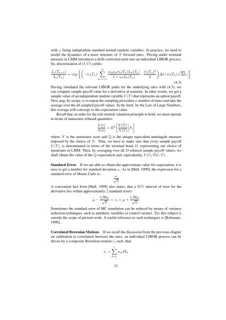
with ɛ i be<strong>in</strong>g <strong>in</strong>dependent st<strong>and</strong>ard normal r<strong>and</strong>om variables. In practice, we need to<br />
<strong>model</strong> <strong>the</strong> dynamics of a tenor structure of N forward rates. Pric<strong>in</strong>g under term<strong>in</strong>al<br />
measure <strong>in</strong> LMM <strong>in</strong>troduces a drift-correction term <strong>in</strong>to an <strong>in</strong>dividual LIBOR process.<br />
So, discretization of (3.17) yields:<br />
L i (T n+1 )<br />
L i (T n )<br />
= exp<br />
{(<br />
−σ i (T n )<br />
N∑<br />
k=i+1<br />
α k ρ ik σ k (T n )L k (T n )<br />
− σ i(T n ) 2 )∆t+σ i (T n ) √ }<br />
∆tɛ i<br />
1 + α k L k (T n ) 2<br />
(4.3)<br />
Hav<strong>in</strong>g simulated <strong>the</strong> relevant LIBOR paths for <strong>the</strong> underly<strong>in</strong>g rates with (4.3), we<br />
can compute sample payoff value for a derivative at maturity. In o<strong>the</strong>r words, we get a<br />
sample value of an <strong>in</strong>dependent r<strong>and</strong>om variable V (T ) that represents an <strong>option</strong> payoff.<br />
Next step, by recipe, is to repeat <strong>the</strong> sampl<strong>in</strong>g procedure n number of times <strong>and</strong> take <strong>the</strong><br />
average over <strong>the</strong> all sampled payoff values. In <strong>the</strong> limit, by <strong>the</strong> Law of Large Numbers,<br />
this average will converge to <strong>the</strong> expectation value.<br />
Recall that, <strong>in</strong> order for <strong>the</strong> risk-neutral <strong>valuation</strong> pr<strong>in</strong>ciple to hold, we must operate<br />
<strong>in</strong> terms of numeraire-rebased quantities:<br />
[ ]<br />
V (t) V (T )<br />
N(t) = EQ N(T ) ∣ F t<br />
where N is <strong>the</strong> numeraire asset <strong>and</strong> Q is <strong>the</strong> unique equivalent mart<strong>in</strong>gale measure<br />
imposed by <strong>the</strong> choice of N. Thus, we have to make sure that every sample payoff<br />
V (T ), is denom<strong>in</strong>ated <strong>in</strong> terms of <strong>the</strong> term<strong>in</strong>al bond D, represent<strong>in</strong>g our choice of<br />
numeraire <strong>in</strong> LMM. Then, by averag<strong>in</strong>g over all D-rebased sample payoff values, we<br />
shall obta<strong>in</strong> <strong>the</strong> value of <strong>the</strong> Q-expectation <strong>and</strong>, equivalently, V (t)/D(t, T ).<br />
St<strong>and</strong>ard Error If we are able to obta<strong>in</strong> <strong>the</strong> approximate value for expectation, it is<br />
easy to get a number for st<strong>and</strong>ard deviation ω. As <strong>in</strong> [Hull, 1999], <strong>the</strong> expression for a<br />
st<strong>and</strong>ard error of Monte Carlo is:<br />
ω<br />
√ n<br />
A convenient fact from [Hull, 1999] also states, that a 95% <strong>in</strong>terval of trust for <strong>the</strong><br />
derivative lies with<strong>in</strong> approximately 2 st<strong>and</strong>ard errors:<br />
µ − 1.96ω √ n<br />
< c t < µ + 1.96ω √ n<br />
Sometimes <strong>the</strong> st<strong>and</strong>ard error of MC simulation can be reduced by means of variance<br />
reduction techniques, such as anti<strong>the</strong>tic variables or control variates. Yet, this subject is<br />
outside <strong>the</strong> scope of present work. A useful reference to such techniques is [Rebonato,<br />
1998].<br />
Correlated Brownian Motions If we recall <strong>the</strong> discussion from <strong>the</strong> previous chapter<br />
on calibration to correlation between <strong>the</strong> rates, an <strong>in</strong>dividual LIBOR process can be<br />
driven by a composite Brownian motion ˆɛ i such, that:<br />
ˆɛ i =<br />
i∑<br />
α ik W k<br />
k=1<br />
31


