sparse grid method in the libor market model. option valuation and the

00 03 02 03 01 03 02 03 00
30 30
20 12 20
30 30
10 21 11 21 10
30 30
20 12 20
30 30
00 03 02 03 01 03 02 03 00
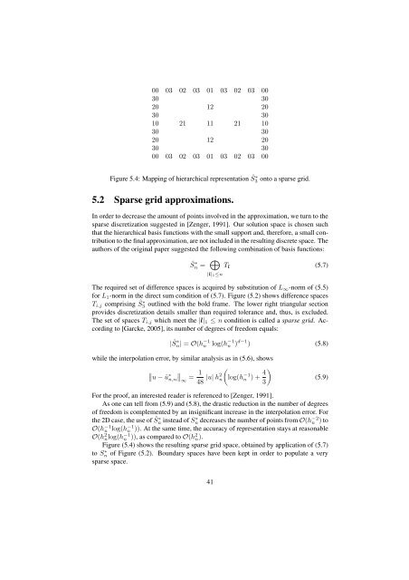
Figure 5.4: Mapping of hierarchical representation Ŝ∗ 3 onto a sparse grid.
5.2 Sparse grid approximations.
In order to decrease the amount of points involved in the approximation, we turn to the
sparse discretization suggested in [Zenger, 1991]. Our solution space is chosen such
that the hierarchical basis functions with the small support and, therefore, a small contribution
to the final approximation, are not included in the resulting discrete space. The
authors of the original paper suggested the following combination of basis functions:
Ŝn ∗ = ⊕
T l (5.7)
|l| 1≤n
The required set of difference spaces is acquired by substitution of L ∞ -norm of (5.5)
for L 1 -norm in the direct sum condition of (5.7). Figure (5.2) shows difference spaces
T i,j comprising Ŝ∗ 3 outlined with the bold frame. The lower right triangular section
provides discretization details smaller than required tolerance and, thus, is excluded.
The set of spaces T i,j which meet the |l| 1 ≤ n condition is called a sparse grid. According
to [Garcke, 2005], its number of degrees of freedom equals:
|Ŝ∗ n| = O(h −1
n
log(h −1
n ) d−1 ) (5.8)
while the interpolation error, by similar analysis as in (5.6), shows
∥
∥u − û ∗ ∥
n,n ∞
= 1 (
48 |u| h2 n log(h −1
n ) + 4 )
3
(5.9)
For the proof, an interested reader is referenced to [Zenger, 1991].
As one can tell from (5.9) and (5.8), the drastic reduction in the number of degrees
of freedom is complemented by an insignificant increase in the interpolation error. For
the 2D case, the use of Ŝ∗ n instead of Sn ∗ decreases the number of points from O(h −2
n ) to
O(h −1
n log(h −1
n )). At the same time, the accuracy of representation stays at reasonable
O(h 2 nlog(h −1
n )), as compared to O(h 2 n).
Figure (5.4) shows the resulting sparse grid space, obtained by application of (5.7)
to Sn ∗ of Figure (5.2). Boundary spaces have been kept in order to populate a very
sparse space.
41