sparse grid method in the libor market model. option valuation and the

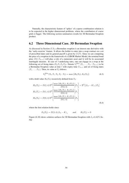
Naturally, the characteristic feature of ’spikes’ of a sparse combination solution is
to be expected in the higher dimensional problems, where the contribution of coarse
grids is bigger. The following section summarizes results for 3D Bermudan Swaption
product.
6.2 Three Dimensional Case. 3D Bermudan Swaption
As discussed in Section (3.3), a Bermudan swaption is an interest rate derivative with
the ’early-exercise’ feature. It allows the holder to enter into a swap contract on a set
of prescribed dates and its general payoff is given by (3.27). Since we are computing
the price of a swaption in the framework of a LIBOR Market Model, the terminal bond
price D(t, T N+1 ) will play a role of a numeraire asset and Q will be its associated
martingale measure. In case of 3 underlying rates, one can engage in a swap at the
following set of fixing dates (T 0 ,T 1 ,T 2 ,T 3 ). Denote Vt
BSw (T t , . . . , T N : T N+1 ) to be
a Bermudan Swaption value at time t with expiry time T N+1 and set of fixing dates
(T t , . . . , T N ). Then, its value at T 0 follows:
V BSw
0 (T 0 , T 1 , T 2 , T 3 : T 4 ) = max ( H 0 (T 0 ), E 0 (T 0 ) ) (6.3)
with a hold value H 0 (T 0 ) recursively defined from T 3 :
[ (
max
H 2 (T 2 ) = D(2, 4) E Q H3 (T 3 ), E 3 (T 3 ) )
]
D(3, 4) ∣ F 2 = E Q[ ]
(L 3 − K) + |F 2
[ (
max
H 1 (T 1 ) = D(1, 4) E Q H2 (T 2 ), E 2 (T 2 ) )
]
D(2, 4) ∣ F 1
[ (
max
H 0 (T 0 ) = D(0, 4) E Q H1 (T 1 ), E 1 (T 1 ) )
]
D(1, 4) ∣ F 0
where the first relation holds since:
E 3 (T 3 ) = D(3, 4) (L 3 − K) +
and H 3 (T 3 ) = 0
(6.4)
Figure (6.10) shows solution surfaces for 3D Bermudan Swaption with L 1 =5.62% fixing:
54