sparse grid method in the libor market model. option valuation and the

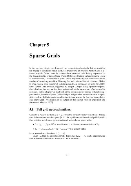
Chapter 5
Sparse Grids
In the previous chapter we discussed two computational methods that are available
for pricing of the claims within the LMM framework. In practice, Monte Carlo is almost
always in favour, since its computational costs are only linearly dependant on
the dimensionality of the problem. Finite Difference Method suffers from the ’curse
of dimensionality’, the number of points grows exponentially with the increase in the
number of underlying variables. This only fact undermines all the nice features FD has
to offer, since a great number of realistic products are contingent on up to 30 LIBOR
rates. Sparse Grid methods, suggested by Zenger [Zenger, 1991], operate on spatial
discretizations that rely on far fewer points and, at the same time, offer reasonable
accuracy. In this chapter we shall look at the common issues related to function approximation,
introduce Sparse Grid technique and postulate results for error analysis.
At the end we shall discuss the combination technique used for function interpolation
on a sparse grid. Presentation of the subject in this chapter relies on exposition and
notation of [Garcke, 2005].
5.1 Full grid approximations.
Consider a PDE of the form Lu = f, subject to certain boundary conditions, defined
on a d-dimensional solution space [0, 1] d . An equidistant d-dimensional grid Ω l could
then be taken as a discrete approximation of such solution space, with :
• l = (l 1 , . . . , l d ) ∈ N d as a multi-index, i.e. discretization resolution of Ω l
• h l := (h l1 , . . . , h ld ) := (2 −l 1
, . . . , 2 −l d
) as a mesh width
in each coordinate direction t ∈ [1 . . . d].
Given Ω l , then the discretized PDE, denoted as L l u l = f l , can be approximated
with either standard basis or hierarchical basis functions.
37