sparse grid method in the libor market model. option valuation and the

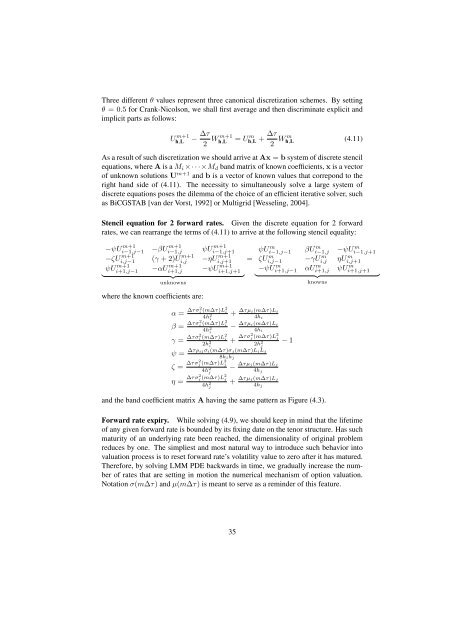
Three different θ values represent three canonical discretization schemes. By setting
θ = 0.5 for Crank-Nicolson, we shall first average and then discriminate explicit and
implicit parts as follows:
U m+1
h,L
− ∆τ
2 W m+1
h,L
= Uh,L m + ∆τ
2 W h,L m (4.11)
As a result of such discretization we should arrive at Ax = b system of discrete stencil
equations, where A is a M i ×· · ·×M d band matrix of known coefficients, x is a vector
of unknown solutions U m+1 and b is a vector of known values that correpond to the
right hand side of (4.11). The necessity to simultaneously solve a large system of
discrete equations poses the dilemma of the choice of an efficient iterative solver, such
as BiCGSTAB [van der Vorst, 1992] or Multigrid [Wesseling, 2004].
Stencil equation for 2 forward rates. Given the discrete equation for 2 forward
rates, we can rearrange the terms of (4.11) to arrive at the following stencil equality:
−ψU m+1
i−1,j−1 −βU m+1
i−1,j ψU m+1
i−1,j+1
−ζU m+1
i,j−1 (γ + 2)U m+1
i,j −ηU m+1
i,j+1
ψU m+1
i+1,j−1 −αU m+1
i+1,j −ψU m+1
i+1,j+1
} {{ }
unknowns
where the known coefficients are:
=
ψUi−1,j−1 m βUi−1,j m −ψUi−1,j+1
m
ζUi,j−1 m −γUi,j m ηUi,j+1
m
−ψUi+1,j−1 m }
αUi+1,j m {{
ψUi+1,j+1
m }
knowns
α = ∆τσ2 i (m∆τ)L2 i
4h 2 i
β = ∆τσ2 i (m∆τ)L2 i
4h 2 i
γ = ∆τσ2 i (m∆τ)L2 i
2h 2 i
+ ∆τµi(m∆τ)Li
4h i
− ∆τµ i(m∆τ)L i
4h i
+ ∆τσ2 j (m∆τ)L2 j
2h 2 j
ψ = ∆τρ ijσ i (m∆τ)σ j (m∆τ)L i L j
8h ih j
ζ = ∆τσ2 j (m∆τ)L2 j
4h 2 j
η = ∆τσ2 j (m∆τ)L2 j
4h 2 j
− ∆τµ j(m∆τ)L j
4h j
+ ∆τµ j(m∆τ)L j
4h j
− 1
and the band coefficient matrix A having the same pattern as Figure (4.3).
Forward rate expiry. While solving (4.9), we should keep in mind that the lifetime
of any given forward rate is bounded by its fixing date on the tenor structure. Has such
maturity of an underlying rate been reached, the dimensionality of original problem
reduces by one. The simpliest and most natural way to introduce such behavior into
valuation process is to reset forward rate’s volatility value to zero after it has matured.
Therefore, by solving LMM PDE backwards in time, we gradually increase the number
of rates that are setting in motion the numerical mechanism of option valuation.
Notation σ(m∆τ) and µ(m∆τ) is meant to serve as a reminder of this feature.
35