sparse grid method in the libor market model. option valuation and the

a good compromise on the size of ɛ are required to capture the reaction of MC option
value to small parameter shifts.
4.2 Finite Difference Method
While Monte Carlo simulation remains the industry’s tool of choice for pricing interest
rate derivatives within LMM framework, the difficulties mentioned above motivate
researchers appeal to alternatives approaches.
d=2
4
3
2
1
0
0
1
2
h
1
}
3
4
} h 2
with:
d=1
h=
L=
m
U h , L
( h 1,h
) t
2
( 2,3) t
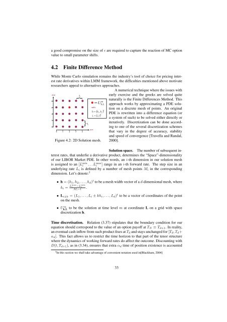
Figure 4.2: 2D Solution mesh.
A numerical technique where the issues with
early exercise and the greeks are solved quite
naturally is the Finite Differences Method. This
approach works by approximating a PDE solution
on a discrete mesh of points. An original
PDE is rewritten into a difference equation (or
a system of such) to be solved either directly or
iteratively. Discretization can be done according
to one of the several discretization schemes
that vary in the degree of accuracy, stability
and speed of convergence [Travella and Randal,
2000].
Solution space. The number of subsequent interest
rates, that underlie a derivative product, determines the “Space”-dimensionality
of our LIBOR Market PDE. In other words, an i-th dimension in our solution mesh
is assigned to an [L min
i . . . L max
i ] range in an i-th forward rate. The step size in an
underlying rate L i is defined by a number of mesh points M i in the corresponding
dimension. Let’s denote: 3
• h = (h 1 , h 2 , . . . , h d ) t to be a mesh width vector of a d-dimensional mesh, where
h i = Lmax i
−L min
i
M i −1
.
• L i±k = (L 1 , . . . , L i ± kh i , . . . , L d ) t to be a vector of coordinates of the point
on the mesh.
• Uh,L m to be the solution at time level m at coordinate L on a grid with space
discretization h.
Time discretisation. Relation (3.37) stipulates that the boundary condition for our
equation should correspond to the value of an option payoff at T N ≡ T d+1 . In reality,
an eventual cash inflow from such product fixes at T d and stays unchanged for [T d , T d +
α d ]. This fact allows us to restrict the time horizon to that part of the tenor structure
where the dynamics of working forward rates do affect the outcome. Discounting with
D(t, T d+1 ), as in (3.34), ensures that extra α d time of position existence is accounted
3 In this section we shall take advantage of convenient notation used in[Blackham, 2004]
33