sparse grid method in the libor market model. option valuation and the

More documents

Recommendations

Info

$Learning LATEX by Doing$

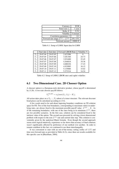
Currency EUR Tenor size α i 1 year Strike K 5.5% Volatility Constant Correlation parameter β 0.1 Forward rate range L min − L max 0%-15% Notional amount 10000 e Table 6.1: Setup of LMM. Input data for LMM Start date End date Forward LIBOR Rate Volatility % T 0 29.07.04 29.07.05 2.423306 0 T 1 29.07.05 29.07.06 3.281384 24.73 T 2 29.07.06 29.07.07 3.931690 22.45 T 3 29.07.07 29.07.08 4.364818 19.36 T 4 29.07.08 29.07.09 4.680236 17.43 T 5 29.07.09 29.07.10 4.933085 16.15 T 6 29.07.10 29.07.11 5.135066 15.02 T 7 29.07.11 29.07.12 5.273314 14.24 Table 6.2: Setup of LMM. LIBOR rates and caplet volatilies 6.1 Two Dimensional Case. 2D Chooser Option A chooser option is a European-style derivative product, whose payoff is determined by (3.28). A two-rate chooser payoff follows: V Cho2D 3 = α 2 (max(L 1 , L 2 ) − K) + All action takes place on a T 0 , ..., T 3 subset of a tenor structure. The relevant discount bond prices can be calculated according to (3.4). A few words need to be said about imposing boundary conditions on 2D solution space for FD. Two of the four boundaries, corresponding to maximum values in underlying rates, are always fixed to the maximum possible payoff value: L max − K. As of the remaining boundaries, with one of the rates being at its minimum L min , there are two possible scenarios. In the first case, solution can be considered fixed to the intrinsic value of the option. The second case proceeds by solving a lower dimensional problem with respect to the non-L min rate and current time step. This solution is conveniently given by the analytical Black formula. Even though the second approach seems more logical intuitively, experience so far shows that accuracy of final solutions wasn’t significantly affected by preference of one method over another. In order to remain confident in this fact, we continued to use them interchangably. It was convenient to start with an out-of-the-money setting (strike of 5.5% and time-zero forward rates as provided in Table (6.2)), since there are results available for this specific case in [Blackham, 2004]. 44
6.1.1 Convergence of MC, Full and Sparse Grid solutions. MC convergence and its standard error are shown in Figure (6.1). Simulation was performed for the maximum of 4, 000, 000 trials, reaching minimum standard error of 0.022. FD solution for full grid discretization was computed for up to discretization level L = 9. Figure (6.1) shows convincing convergence behavior of simulated solution Level of Discretization 6 6.5 7 7.5 8 8.5 9 10.2 MC Simulation Value+Std.Error Full-Grid FD value 10.15 10.1 Option price 10.05 10 9.95 9.9 9.85 500000 1e+006 1.5e+006 2e+006 2.5e+006 3e+006 3.5e+006 4e+006 Number of MC simulations Figure 6.1: 2D Chooser Option. MC vs. FD Convergence. and full-grid FD, providing accurate reference values for further tests. For our sparse approximation experiments we have used a classical sparse grid (a.k.a ”maximumnorm-based” type) and a basic combination technique, both described in the previous chapter. Table (6.3) and Figure (6.2) give idea of FD convergence on full and sparse grids 2 : Level Full grid Execution Sparse Grid Execution Full grid Sparse grid solution time(sec.) solution time(sec.) points count points count 5 10.5969 1.5 11.351 0.36 1089 257 6 10.1755 6.6 11.477 0.88 4225 577 7 10.0964 30.1 9.8731 2.16 16641 1281 8 10.0762 176.4 10.005 5.18 66049 2817 9 10.0762 651.4 10.165 12.89 263169 6145 10 10.153 31.64 1050625 13313 11 9.998 74.86 4198401 28673 Table 6.3: 2D Chooser. Convergence values for full and sparse grid solutions. 2 The execution time for sparse grid technique does not include interpolation procedure 45
Page 1 and 2: SPARSE GRID METHOD IN THE LIBOR MAR
Page 3 and 4: Acknowledgements This project would
Page 5 and 6: 6.3.1 Valuation Results. . . . . .
Page 7 and 8: 6.18 2D Digital Option. Full and sp
Page 9 and 10: Chapter 1 Introduction The modern f
Page 11 and 12: Chapter 2 Asset Pricing Overview Th
Page 13 and 14: Risk-Neutral Pricing Another import
Page 15 and 16: S 0 u d u S 0 S u 2 0 Su 3 0 S du 2
Page 17 and 18: or log(S T ) d −→ log(S 0 ) +
Page 19 and 20: There is an important difference be
Page 21 and 22: Delta. In order to set up a riskfre
Page 23 and 24: Theorem 2.3.2. Let W P (t) = (W1 P
Page 25 and 26: Chapter 3 LIBOR Market Model Having
Page 27 and 28: The right-hand side of the equality
Page 29 and 30: At this point of the text all neces
Page 31 and 32: pays off at expiry. Conveniently, t
Page 33 and 34: 1. Tenor structure of N interest ra
Page 35 and 36: and weight factor parts from the co
Page 37 and 38: we can substitute into the equation
Page 39 and 40: with ɛ i being independent standar
Page 41 and 42: a good compromise on the size of ɛ
Page 43 and 44: Three different θ values represent
Page 45 and 46: Chapter 5 Sparse Grids In the previ
Page 47 and 48: T 0 , 0 T 0 , 1 T 0 , 2 T 0 , 3 |i|
Page 49 and 50: 00 03 02 03 01 03 02 03 00 30 30 20
Page 51: Chapter 6 Numerical Results. Valuat
Page 55 and 56: Full Solution. Level 6 Option Price
Page 57 and 58: 6.1.2 Discussion: Convergence of Pr
Page 59 and 60: 1 Full Delta Value Sparse Delta Val
Page 61 and 62: 0.03 0.025 Full vega Value Sparse v
Page 63 and 64: L1=5.62% Sparse Solution Swaption P
Page 65 and 66: Level L 2 =1.87% L 2 =1.875% L 2 =5
Page 67 and 68: Figures (6.14) and (6.15) show the
Page 69 and 70: 6.3 Discontinuous Payoff. 2D Digita
Page 71 and 72: Level L 1 =3.75% L 1 =4.68% L 1 =5.
Page 73 and 74: Figures (6.21) and (6.22) show the
Page 75 and 76: Chapter 7 Conclusion and Future Wor
Page 77 and 78: Appendix A Implementation Details I
Page 79: A. Klimke. Piecewise multilinear sp

sparse grid method in the libor market model. option valuation and the

You also want an ePaper? Increase the reach of your titles

Delete template?

Save as template?