pdf download - Software and Computer Technology - TU Delft

5.4 MBD Implementation 1
Diagnosing the Beam Propeller Movement
of the Frontal Stand
(a) One control loop
(b) Two nested control loops
(c) Three nested control loops
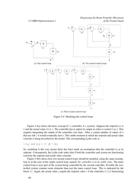
Figure 5.4: Modeling the control loops
Figure 5.4(a) shows the basic concept (C = controller, S = system). Suppose the setpoint (A) is
H and the actual value (B) is L. The controller has to adjust its output in order to control B to H. This
requires integrating the output of the controller over time. After a certain number of values of B
that are still L it would eventually turn H. This stable moment at which the setpoint and actual value
coincide is being described by the model. The corresponding Lydia code is:
( h_c and h_s ) => (B = A);
So, modeling it this way means there has been made an assumption that the controller is at its
setpoint. Consequently, the Lydia code states that if both the controller and system are functioning
correctly the setpoint and actual value coincide.
Figure 5.4(b) shows how two nested control loops should be modeled, using the same assumption
as in the case of the single control loop, namely the controller is in its stable state. The inner
control loop is now part of the system being controlled by the second controller. Possibly the controlled
system contains more elements than just the inner control loop. This is indicated by the
block S2. Again, the actual value Q equals the setpoint value P if the controller (C2) is functioning
60