SPICE-Simulation using LTspice IV
SPICE-Simulation using LTspice IV
SPICE-Simulation using LTspice IV

You also want an ePaper? Increase the reach of your titles
YUMPU automatically turns print PDFs into web optimized ePapers that Google loves.
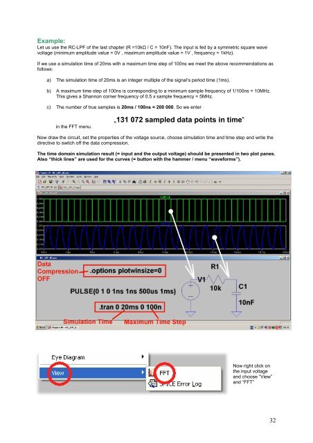
Example:<br />
Let us use the RC-LPF of the last chapter (R =10k / C = 10nF). The input is fed by a symmetric square wave<br />
voltage (minimum amplitude value = 0V , maximum amplitude value = 1V , frequency = 1kHz).<br />
If we use a simulation time of 20ms with a maximum time step of 100ns we meet the above recommendations as<br />
follows:<br />
a) The simulation time of 20ms is an integer multiple of the signal’s period time (1ms).<br />
b) A maximum time step of 100ns is corresponding to a minimum sample frequency of 1/100ns = 10MHz.<br />
This gives a Shannon corner frequency of 0.5 x sample frequency = 5MHz.<br />
c) The number of true samples is 20ms / 100ns = 200 000. So we enter<br />
in the FFT menu.<br />
„131 072 sampled data points in time“<br />
Now draw the circuit, set the properties of the voltage source, choose simulation time and time step and write the<br />
directive to switch off the data compression.<br />
The time domain simulation result (= input and the output voltage) should be presented in two plot panes.<br />
Also “thick lines” are used for the curves (= button with the hammer / menu “waveforms”).<br />
Now right click on<br />
the input voltage<br />
and choose “View”<br />
and “FFT”<br />
32