Gaming the Float: How Managers Respond to EPS-based Incentives

More documents

Recommendations

Info

Finally, TSM has implications for a variety of per-share metrics such as analyst dispersion and forecast error. In this sense, our findings compliment Dechow and You (2012), in which the authors make the observation that the precision of an EPS number is greater for higher levels of EPS. 10 We show in Section 3.3 that the scale invariance of analysts’ forecast errors (Degeorge et al. (1999), Cheong and Thomas (2011), and Ball (2011)) is the expected endogenous outcome of target size management. Our paper proceeds as follows: Section 2 motivates our hypothesis and describes the mechanism we test. Section 3 describes the data and empirical results. Section 3.3 discusses the implications of our findings, and Section 4 concludes. 2 Discussion and Hypothesis Development The convention of rounding EPS to the nearest penny creates a range of net income that will generate a given EPS number. The size of this range is determined by the number of shares outstanding. Specifically, the range of net income that meets expectations is: (E[EP S] ∗ s − s s 200 , E[EP S] ∗ s + 200 ), where E[EP S] is the analysts’ EPS expectation and s is the number of shares outstanding. The expected Net Income, E[EP S] ∗ s, is the total earnings implied by the per share forecast and is the midpoint of this range. The highest and lowest earnings that will round to the forecast are determined by s. At a maximum, each share’s 1 worth of earnings will be rounded by half a penny (or in dollar terms, 200 ). For example, Microsoft Corp. has roughly 8 billion shares outstanding. So, in any given quarter the total size of their earnings target is 80 million dollars, ± 40 million centered around the amount of total earnings implied by the forecast. In dollar terms this amount might seem large, but relative to the magnitude of the firm’s earnings, perhaps less so. The size of the earnings target relative to the size of the firm’s total earnings is ± 0.5 E[|EP S|] %. The average firm in our sample has EPS of $0.20. So, the typical firm will meet the earnings forecast by producing earnings within ±2.50% of expected earnings. This amount of flexibility might be considered large by some managers and small by others. For example, 2.50% may be relatively large for a firm with stable business fundamentals and predictable net income. However, a manager whose compensation is highly concave in earnings surprises may consider this range to be small. Managers have flexibility over the size of this earnings target. In dollar terms, the size of the target is fixed solely by the number of shares. If the manager prefers an earnings target twice as large, she can simply double the number of shares outstanding. Because the size of the earnings target measured in dollars is fixed, 10 In the next section, we show that the target size as a percentage of the firm’s expected net income equals one-half of the inverse of EPS. 6
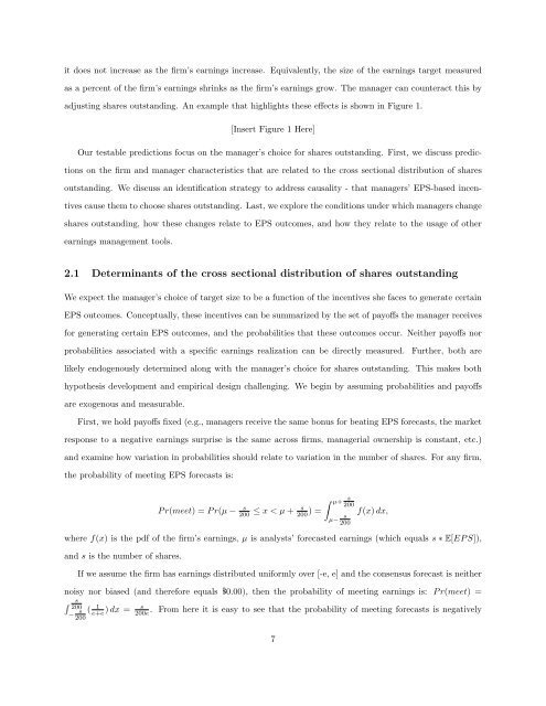
it does not increase as the firm’s earnings increase. Equivalently, the size of the earnings target measured as a percent of the firm’s earnings shrinks as the firm’s earnings grow. The manager can counteract this by adjusting shares outstanding. An example that highlights these effects is shown in Figure 1. [Insert Figure 1 Here] Our testable predictions focus on the manager’s choice for shares outstanding. First, we discuss predictions on the firm and manager characteristics that are related to the cross sectional distribution of shares outstanding. We discuss an identification strategy to address causality - that managers’ EPS-based incentives cause them to choose shares outstanding. Last, we explore the conditions under which managers change shares outstanding, how these changes relate to EPS outcomes, and how they relate to the usage of other earnings management tools. 2.1 Determinants of the cross sectional distribution of shares outstanding We expect the manager’s choice of target size to be a function of the incentives she faces to generate certain EPS outcomes. Conceptually, these incentives can be summarized by the set of payoffs the manager receives for generating certain EPS outcomes, and the probabilities that these outcomes occur. Neither payoffs nor probabilities associated with a specific earnings realization can be directly measured. Further, both are likely endogenously determined along with the manager’s choice for shares outstanding. This makes both hypothesis development and empirical design challenging. We begin by assuming probabilities and payoffs are exogenous and measurable. First, we hold payoffs fixed (e.g., managers receive the same bonus for beating EPS forecasts, the market response to a negative earnings surprise is the same across firms, managerial ownership is constant, etc.) and examine how variation in probabilities should relate to variation in the number of shares. For any firm, the probability of meeting EPS forecasts is: P r(meet) = P r(µ − ∫ s µ+ s 200 ≤ x < µ + s 200 ) = 200 µ− s 200 f(x) dx, where f(x) is the pdf of the firm’s earnings, µ is analysts’ forecasted earnings (which equals s ∗ E[EP S]), and s is the number of shares. If we assume the firm has earnings distributed uniformly over [-e, e] and the consensus forecast is neither noisy nor biased (and therefore equals $0.00), then the probability of meeting earnings is: P r(meet) = ∫ s 200 − s 200 ( 1 e+e ) dx = s 200e . From here it is easy to see that the probability of meeting forecasts is negatively 7
Page 1 and 2: Gaming the Float: How Managers Resp
Page 3 and 4: earnings will choose more shares ou
Page 5: targets. Managers change the target
Page 9 and 10: meeting that forecast. This leads t
Page 11 and 12: 2.2 Time series determinants of sha
Page 13 and 14: ealized but before they are reporte
Page 15 and 16: A and incentive compensation in Pan
Page 17 and 18: elationship between incentive compe
Page 19 and 20: the view that increases in forecast
Page 21 and 22: In columns 2 and 3, we measure our
Page 23 and 24: atypical amount. In Table 9, we rep
Page 25 and 26: price levels observed in the data.
Page 27 and 28: management tools. 27
Page 29 and 30: De Angelis, D. and Y. Grinstein (20
Page 31 and 32: A Appendix We show that a drop in a
Page 33 and 34: Figure 1: Example of the relationsh
Page 35 and 36: Figure 3: Median Shares Outstanding
Page 37 and 38: Table 2: Determinants of Shares Out
Page 39 and 40: Table 4: Shares Outstanding: First
Page 41 and 42: Table 6: Changes in Shares Outstand
Page 43 and 44: Table 8: Changes in Shares and Acco

Gaming the Float: How Managers Respond to EPS-based Incentives

You also want an ePaper? Increase the reach of your titles

Delete template?

Save as template?