Astronomical Spectroscopy - Physics - University of Cincinnati
Astronomical Spectroscopy - Physics - University of Cincinnati
Astronomical Spectroscopy - Physics - University of Cincinnati
You also want an ePaper? Increase the reach of your titles
YUMPU automatically turns print PDFs into web optimized ePapers that Google loves.
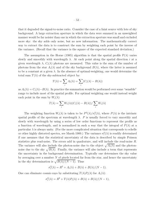
– 53 –<br />
that it degraded the signal-to-noise ratio. Consider the case <strong>of</strong> a faint source with lots <strong>of</strong> sky<br />
background. A large extraction aperture in which the data were summed in an unweighted<br />
manner would be far noisier than one in which the extraction aperture was small and excluded<br />
more sky: the sky adds only noise, but no new information. The mathematically correct<br />
way to extract the data is to construct the sum by weighting each point by the inverse <strong>of</strong><br />
the variance. (Recall that the variance is the square <strong>of</strong> the expected standard deviation.)<br />
The assumption in the Horne (1985) algorithm is that the spatial pr<strong>of</strong>ile P(λ) varies<br />
slowly and smoothly with wavelength λ. At each point along the spatial direction i at a<br />
given wavelength λ, C i (λ) photons are measured. This value is the sum <strong>of</strong> the number <strong>of</strong><br />
photons from the star A i (λ) and <strong>of</strong> the sky background B(λ), where the latter is assumed<br />
to be a constant at a given λ. In the absence <strong>of</strong> optimal-weighting, one would determine the<br />
total sum T(λ) <strong>of</strong> the sky-subtracted object by:<br />
T(λ) = ∑ i<br />
A i (λ) = ∑ i<br />
(C i (λ) − B(λ))<br />
as A i (λ) = C i (λ)−B(λ). In practice the summation would be performed over some “sensible”<br />
range to include most <strong>of</strong> the spatial pr<strong>of</strong>ile. For optimal weighting one would instead weight<br />
each point in the sum by W i (λ):<br />
T(λ) = ∑ i<br />
W i (λ)(C i (λ) − B(λ))/ ∑ i<br />
W i (λ)<br />
The weighting function W i (λ) is taken to be P 2 (λ)/σi 2 (λ), where P(λ) is the intrinsic<br />
spatial pr<strong>of</strong>ile <strong>of</strong> the spectrum at wavelength λ. P is usually forced to vary smoothly and<br />
slowly with wavelength by using a series <strong>of</strong> low order functions to represent the pr<strong>of</strong>ile as<br />
a function <strong>of</strong> wavelength, and is normalized in such a way that the integral <strong>of</strong> P(λ) at a<br />
particular λ is always unity. (For the more complicated situation that corresponds to echelle<br />
or other highly distorted spectra, see Marsh 1989.) The variance σi 2 (λ) is readily determined<br />
if one assumes that the statistical uncertainty <strong>of</strong> the data is described by simple Poisson<br />
statistics plus read-noise. The errors add in quadrature, and will include the read-noise R.<br />
The variance will also include the photon-noise due to the object √ A i (λ) and the photonnoise<br />
due to the sky √ B(λ). Finally, the variance will also include a term that represents<br />
the uncertainty in the background determination. Typically one determines the sky value<br />
by averaging over a number N <strong>of</strong> pixels located far from the star, and hence the uncertainty<br />
in the sky determination is √ B(λ)/(N − 1). Thus<br />
σ 2 i (λ) = R2 + A i (λ) + B(λ) + B(λ)/(N − 1).<br />
One can eliminate cosmic-rays by substituting T(λ)P i (λ) for A i (λ):<br />
σ 2 i (λ) = R 2 + T(λ)P i (λ) + B(λ) + B(λ)/(N − 1),


