1000 Hydraulics Chapter - Ministry of Transportation
1000 Hydraulics Chapter - Ministry of Transportation
1000 Hydraulics Chapter - Ministry of Transportation

You also want an ePaper? Increase the reach of your titles
YUMPU automatically turns print PDFs into web optimized ePapers that Google loves.
SUPPLEMENT TO TAC GEOMETRIC DESIGN GUIDE<br />
MoT Section 1020 TAC Section Not Applicable<br />
BC MoT<br />
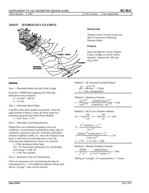
1020.07 HYDROLOGY EXAMPLE<br />
Background<br />
Thames Creek is located on the east<br />
side <strong>of</strong> Vancouver Island near<br />
Denman Island.<br />
Problem<br />
Since the highway crosses Thames<br />
Creek, a bridge or culvert will be<br />
required. Estimate the 200-year<br />
(Q 200 ) flow.<br />
Solution<br />
Step 1 - Determine Basin Size and Creek Length<br />
From the 1:50000 scale mapping, the following<br />
dimensions were measured:<br />
A = 6.6 km 2 = 660 ha<br />
L = 8.2 km<br />
Step 2 - Determine Basin Slope<br />
A pr<strong>of</strong>ile <strong>of</strong> the main channel was plotted. Since the<br />
upper portion <strong>of</strong> basin is steep, the basin slope was<br />
estimated using the Equivalent Slope Method.<br />
s = 0.051 m/m = 5.1%<br />
Step 3 - Determine Land Characteristics<br />
Design flows are estimated assuming worst case<br />
conditions. Considerations include basin slope, type <strong>of</strong><br />
vegetation, recurrence intervals, snowmelt, antecedent<br />
moisture condition (AMC) etc. Since the Thames Creek<br />
basin is relatively low with light forest cover, the<br />
following land characteristic values were selected:<br />
r = 0.60, deciduous timber land<br />
CN = 85, forest land with good cover, Hydrologic<br />
Soil Group C, AMC III<br />
C = 0.40, flat, forested<br />
Step 4 - Determine Time <strong>of</strong> Concentration<br />
There are numerous ways <strong>of</strong> estimating the time <strong>of</strong><br />
concentration (t c ). A few different methods will be used<br />
and an “average” value will be selected.<br />
Method 1 - BC Rational Formula Method<br />
A = 66 . km = 2.6km<br />
t c = 3.6hr (interpolated)<br />
2<br />
Method 2 - Hathaway Formula<br />
t = (rL) 0.467 0.467<br />
(( 0. 60)(8.<br />
2km))<br />
c<br />
= = 2.6hr<br />
0234 .<br />
0.234<br />
165 . s 1. 65( 0.<br />
051m/m)<br />
Method 3 - SCS Curve Number Method<br />
S = 254( 100<br />
CN − 1) = 254( 100 − 1)<br />
= 44.8<br />
CN<br />
85<br />
0.8<br />
0.7<br />
T = L ( 0.<br />
039SCN<br />
+1)<br />
L<br />
0.5<br />
735 s<br />
0.8<br />
( 8200m)<br />
( 0. 039( 44.8) + 1)<br />
=<br />
05 .<br />
735(.<br />
51%)<br />
t c = 1.7T L = 1.7(1.7hr) = 2.8hr<br />
07 .<br />
= 17 . hr<br />
Method 4 - Bransby Williams Formula<br />
t = 0.605L 0605 . ( 82 . km)<br />
c = = 30 . hr<br />
0.2 0.1 0.2 2 01 .<br />
s A (5.1%) ( 66 . km )<br />
Taking an “average”, it is assumed that t c =3 hours.<br />
Page 1020-6 June, 2007