- Page 1: PROCEEDINGS OF THEINTERNATIONAL WOR
- Page 5 and 6: ContentsPrefaceiiiPlenary TalksYaro
- Page 7 and 8: ContentsviiFuh-Hwa Franklin Liu, Ch
- Page 9: PLENARY TALKS
- Page 12 and 13: 4 Yaroslav D. Sergeyevto work with
- Page 15: EXTENDED ABSTRACTS
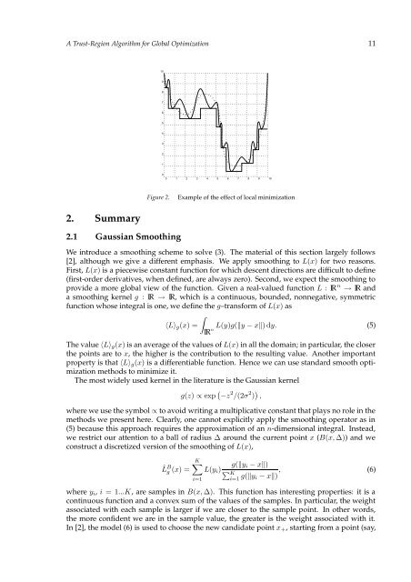
- Page 20 and 21: 12 Bernardetta Addis and Sven Leyff
- Page 22 and 23: 14 Bernardetta Addis and Sven Leyff
- Page 24 and 25: 16 Bernardetta Addis, Marco Locatel
- Page 26 and 27: 18 April K. Andreas and J. Cole Smi
- Page 28 and 29: 20 April K. Andreas and J. Cole Smi
- Page 30 and 31: 22 April K. Andreas and J. Cole Smi
- Page 32 and 33: 24 Charles Audet, Pierre Hansen, an
- Page 34 and 35: 26 Charles Audet, Pierre Hansen, an
- Page 36 and 37: 28 Charles Audet, Pierre Hansen, an
- Page 38 and 39: 30 János Balogh, József Békési,
- Page 40 and 41: 32 János Balogh, József Békési,
- Page 42 and 43: 34 János Balogh, József Békési,
- Page 44 and 45: 36 Balázs Bánhelyi, Tibor Csendes
- Page 47 and 48: Proceedings of GO 2005, pp. 39 - 45
- Page 49 and 50: MGA Pruning Technique 41Figure 1. A
- Page 51 and 52: MGA Pruning Technique 43O(n) = k 2
- Page 53: MGA Pruning Technique 45one), while
- Page 56 and 57: 48 Edson Tadeu Bez, Mirian Buss Gon
- Page 58 and 59: 50 Edson Tadeu Bez, Mirian Buss Gon
- Page 60 and 61: 52 Edson Tadeu Bez, Mirian Buss Gon
- Page 62 and 63: 54 R. Blanquero, E. Carrizosa, E. C
- Page 64 and 65: 56 R. Blanquero, E. Carrizosa, E. C
- Page 66 and 67: 58 Sándor Bozókiwhere for any i,
- Page 68 and 69:
60 Sándor Bozóki[6] Budescu, D.V.
- Page 70 and 71:
62 Emilio Carrizosa, José Gordillo
- Page 72 and 73:
64 Emilio Carrizosa, José Gordillo
- Page 75 and 76:
Proceedings of GO 2005, pp. 67 - 69
- Page 77:
Globally optimal prototypes 69Refer
- Page 80 and 81:
72 Leocadio G. Casado, Eligius M.T.
- Page 82 and 83:
874 Leocadio G. Casado, Eligius M.T
- Page 84 and 85:
76 Leocadio G. Casado, Eligius M.T.
- Page 86 and 87:
78 András Erik Csallner, Tibor Cse
- Page 88 and 89:
80 András Erik Csallner, Tibor Cse
- Page 90 and 91:
82 Tibor Csendes, Balázs Bánhelyi
- Page 92 and 93:
84 Tibor Csendes, Balázs Bánhelyi
- Page 94 and 95:
86 Bernd DachwaldFor spacecraft wit
- Page 96 and 97:
88 Bernd Dachwaldcurrent target sta
- Page 98 and 99:
90 Bernd Dachwaldreference launch d
- Page 100 and 101:
92 Mirjam Dür and Chris TofallisMo
- Page 102 and 103:
94 Mirjam Dür and Chris Tofallis2.
- Page 104 and 105:
96 Mirjam Dür and Chris Tofallis[3
- Page 106 and 107:
98 José Fernández and Boglárka T
- Page 108 and 109:
100 José Fernández and Boglárka
- Page 110 and 111:
102 José Fernández and Boglárka
- Page 112 and 113:
104 Erika R. Frits, Ali Baharev, Zo
- Page 114 and 115:
106 Erika R. Frits, Ali Baharev, Zo
- Page 116 and 117:
108 Erika R. Frits, Ali Baharev, Zo
- Page 118 and 119:
110 Juergen Garloff and Andrew P. S
- Page 120 and 121:
112 Juergen Garloff and Andrew P. S
- Page 123 and 124:
Proceedings of GO 2005, pp. 115 - 1
- Page 125 and 126:
Global multiobjective optimization
- Page 127 and 128:
Global multiobjective optimization
- Page 129 and 130:
Proceedings of GO 2005, pp. 121 - 1
- Page 131 and 132:
Conditions for ε-Pareto Solutions
- Page 133:
Conditions for ε-Pareto Solutions
- Page 136 and 137:
128 Eligius M.T. Hendrix1.1 Effecti
- Page 138 and 139:
130 Eligius M.T. Hendrix4h(x)3.532.
- Page 140 and 141:
132 Eligius M.T. Hendrixneighbourho
- Page 142 and 143:
134 Kenneth Holmströmcomputed by R
- Page 144 and 145:
136 Kenneth Holmströmα(x) =∑i=1
- Page 146 and 147:
138 Kenneth HolmströmGL-step Phase
- Page 148 and 149:
140 Kenneth Holmströmsurrogate mod
- Page 150 and 151:
142 Dario Izzo and Mihály Csaba Ma
- Page 152 and 153:
144 Dario Izzo and Mihály Csaba Ma
- Page 154 and 155:
146 Dario Izzo and Mihály Csaba Ma
- Page 156 and 157:
148 Leo Liberti and Milan DražićV
- Page 158 and 159:
150 Leo Liberti and Milan Dražićs
- Page 161 and 162:
Proceedings of GO 2005, pp. 153 - 1
- Page 163 and 164:
Set-covering based p-center problem
- Page 165 and 166:
Set-covering based p-center problem
- Page 167 and 168:
Proceedings of GO 2005, pp. 159 - 1
- Page 169 and 170:
On the Solution of Interplanetary T
- Page 171 and 172:
On the Solution of Interplanetary T
- Page 173 and 174:
Proceedings of GO 2005, pp. 165 - 1
- Page 175 and 176:
Parametrical approach for studying
- Page 177 and 178:
Parametrical approach for studying
- Page 179 and 180:
Proceedings of GO 2005, pp. 171 - 1
- Page 181 and 182:
An Interval Branch-and-Bound Algori
- Page 183 and 184:
An Interval Branch-and-Bound Algori
- Page 185 and 186:
Proceedings of GO 2005, pp. 177 - 1
- Page 187 and 188:
A New approach to the Studyof the S
- Page 189:
A New approach to the Studyof the S
- Page 192 and 193:
184 Katharine M. Mullen, Mikas Veng
- Page 194 and 195:
186 Katharine M. Mullen, Mikas Veng
- Page 196 and 197:
188 Katharine M. Mullen, Mikas Veng
- Page 198 and 199:
190 Niels J. Olieman and Eligius M.
- Page 200 and 201:
192 Niels J. Olieman and Eligius M.
- Page 202 and 203:
194 Niels J. Olieman and Eligius M.
- Page 204 and 205:
196 Andrey V. Orlovwhere A is (m 1
- Page 206 and 207:
198 Andrey V. OrlovStep 4. Beginnin
- Page 208 and 209:
200 Blas Pelegrín, Pascual Fernán
- Page 210 and 211:
202 Blas Pelegrín, Pascual Fernán
- Page 212 and 213:
204 Blas Pelegrín, Pascual Fernán
- Page 214 and 215:
206 Blas Pelegrín, Pascual Fernán
- Page 216 and 217:
208 Deolinda M. L. D. Rasteiro and
- Page 218 and 219:
210 Deolinda M. L. D. Rasteiro and
- Page 220 and 221:
212 Deolinda M. L. D. Rasteiro and
- Page 222 and 223:
214 José-Oscar H. Sendín, Antonio
- Page 224 and 225:
216 José-Oscar H. Sendín, Antonio
- Page 226 and 227:
218 José-Oscar H. Sendín, Antonio
- Page 228 and 229:
220 Ya. D. Sergeyev and D. E. Kvaso
- Page 230 and 231:
222 Ya. D. Sergeyev and D. E. Kvaso
- Page 232 and 233:
224 Ya. D. Sergeyev and D. E. Kvaso
- Page 234 and 235:
226 J. Cole Smith, Fransisca Sudarg
- Page 236 and 237:
228 J. Cole Smith, Fransisca Sudarg
- Page 238 and 239:
230 J. Cole Smith, Fransisca Sudarg
- Page 240 and 241:
232 Fazil O. Sonmezcost of a config
- Page 242 and 243:
234 Fazil O. Sonmezhere f h is the
- Page 244 and 245:
236 Fazil O. SonmezThe optimal shap
- Page 246 and 247:
238 Alexander S. StrekalovskyDevelo
- Page 249 and 250:
Proceedings of GO 2005, pp. 241 - 2
- Page 251 and 252:
PSfrag replacementsPruning a box fr
- Page 253 and 254:
Pruning a box from Baumann point in
- Page 255 and 256:
Proceedings of GO 2005, pp. 247 - 2
- Page 257 and 258:
A Hybrid Multi-Agent Collaborative
- Page 259 and 260:
A Hybrid Multi-Agent Collaborative
- Page 261 and 262:
Proceedings of GO 2005, pp. 253 - 2
- Page 263:
Improved lower bounds for optimizat
- Page 266 and 267:
258 Graham R. Wood, Duangdaw Sirisa
- Page 268 and 269:
260 Graham R. Wood, Duangdaw Sirisa
- Page 270 and 271:
262 Graham R. Wood, Duangdaw Sirisa
- Page 272 and 273:
264 Yinfeng Xu and Wenqiang Daiopti
- Page 274 and 275:
266 Yinfeng Xu and Wenqiang DaiThe
- Page 277 and 278:
Author IndexAddis, BernardettaDipar
- Page 279:
Author Index 271Nasuto, S.J.Departm