View - Universidad de Almería

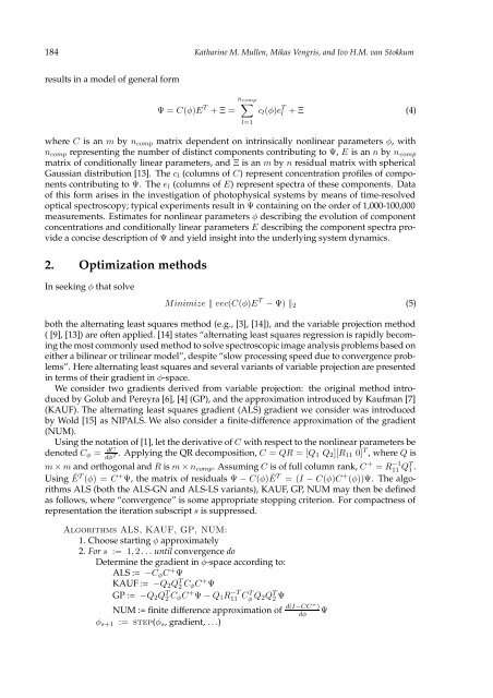
184 Katharine M. Mullen, Mikas Vengris, and Ivo H.M. van Stokkumresults in a model of general formΨ = C(φ)E T + Ξ =n∑ compl=1c l (φ)e T l + Ξ (4)where C is an m by n comp matrix dependent on intrinsically nonlinear parameters φ, withn comp representing the number of distinct components contributing to Ψ, E is an n by n compmatrix of conditionally linear parameters, and Ξ is an m by n residual matrix with sphericalGaussian distribution [13]. The c l (columns of C) represent concentration profiles of componentscontributing to Ψ. The e l (columns of E) represent spectra of these components. Dataof this form arises in the investigation of photophysical systems by means of time-resolvedoptical spectroscopy; typical experiments result in Ψ containing on the order of 1,000-100,000measurements. Estimates for nonlinear parameters φ describing the evolution of componentconcentrations and conditionally linear parameters E describing the component spectra providea concise description of Ψ and yield insight into the underlying system dynamics.2. Optimization methodsIn seeking φ that solveMinimize ‖ vec(C(φ)E T − Ψ) ‖ 2 (5)both the alternating least squares method (e.g., [3], [14]), and the variable projection method( [9], [13]) are often applied. [14] states “alternating least squares regression is rapidly becomingthe most commonly used method to solve spectroscopic image analysis problems based oneither a bilinear or trilinear model”, despite “slow processing speed due to convergence problems”.Here alternating least squares and several variants of variable projection are presentedin terms of their gradient in φ-space.We consider two gradients derived from variable projection: the original method introducedby Golub and Pereyra [6], [4] (GP), and the approximation introduced by Kaufman [7](KAUF). The alternating least squares gradient (ALS) gradient we consider was introducedby Wold [15] as NIPALS. We also consider a finite-difference approximation of the gradient(NUM).Using the notation of [1], let the derivative of C with respect to the nonlinear parameters bedenoted C φ = dC . Applying the QR decomposition, C = QR = [Qdφ T 1 Q 2 ][R 11 0] T , where Q ism × m and orthogonal and R is m × n comp . Assuming C is of full column rank, C + = R11 −1 QT 1 .Using ÊT (φ) = C + Ψ, the matrix of residuals Ψ − C(φ)ÊT = (I − C(φ)C + (φ))Ψ. The algorithmsALS (both the ALS-GN and ALS-LS variants), KAUF, GP, NUM may then be definedas follows, where “convergence” is some appropriate stopping criterion. For compactness ofrepresentation the iteration subscript s is suppressed.Algorithms ALS, KAUF, GP, NUM:1. Choose starting φ approximately2. For s := 1, 2 . . . until convergence doDetermine the gradient in φ-space according to:ALS := −C φ C + ΨKAUF := −Q 2 Q T 2 C φC + ΨGP := −Q 2 Q T 2 C φC + Ψ − Q 1 R11 −T CT φ Q 2Q T 2 ΨNUM := finite difference approximation of d(I−CC+ )dφΨφ s+1 := step(φ s , gradient, . . .)