View - Universidad de Almería

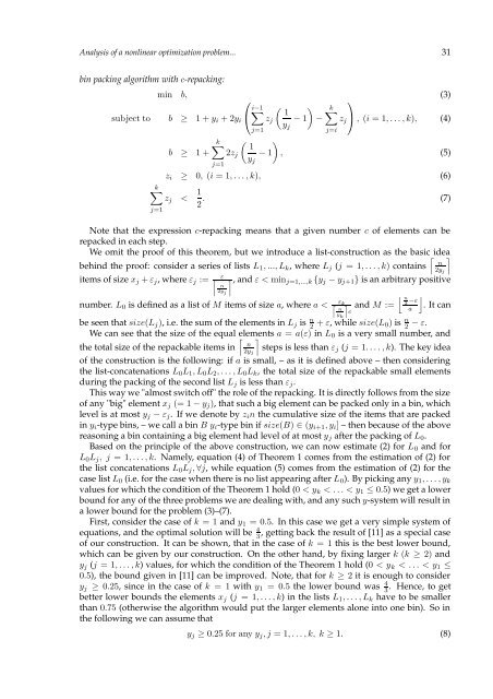
Analysis of a nonlinear optimization problem... 31bin packing algorithm with c-repacking:min b, (3)⎛⎞∑i−1( )subject to b ≥ 1 + y i + 2y i⎝ 1k∑z j − 1 − z j⎠ , (i = 1, . . . , k), (4)y jb ≥ 1 +j=1j=ik∑( ) 12z j − 1 , (5)y jj=1z i ≥ 0, (i = 1, . . . , k), (6)k∑z j < 1 2 . (7)j=1Note that the expression c-repacking means that a given number c of elements can berepacked in each step.We omit the proof of this theorem, but we introduce a list-construction as the basic ideabehind the proof: consider a series of lists L 1 , ..., L k , where L j (j = 1, . . . , k) containsitems of size x j + ε j , where ε j :=⌈ ⌉n2y j‰ ε ı, and ε < min j=1,...,k {y j − y j+1 } is an arbitrary positiven2y j⌊number. L 0 is defined as a list of M items of size a, where a < l ε kmand M := n2 −εncay kbe seen that size(L j ), i.e. the sum of the elements in L j is n 2 + ε, while size(L 0) is n 2 − ε.⌋. It canWe can see that the size of the equal elements a = a(ε) in L 0 is a very small number, andthe total size of the repackable items in⌈ ⌉n2y jsteps is less than ε j (j = 1. . . . , k). The key ideaof the construction is the following: if a is small, – as it is defined above – then consideringthe list-concatenations L 0 L 1 , L 0 L 2 , . . . , L 0 L k , the total size of the repackable small elementsduring the packing of the second list L j is less than ε j .This way we "almost switch off" the role of the repacking. It is directly follows from the sizeof any "big" element x j (= 1 − y j ), that such a big element can be packed only in a bin, whichlevel is at most y j − ε j . If we denote by z i n the cumulative size of the items that are packedin y i -type bins, – we call a bin B y i -type bin if size(B) ∈ (y i+1 , y i ] – then because of the abovereasoning a bin containing a big element had level of at most y j after the packing of L 0 .Based on the principle of the above construction, we can now estimate (2) for L 0 and forL 0 L j , j = 1, . . . , k. Namely, equation (4) of Theorem 1 comes from the estimation of (2) forthe list concatenations L 0 L j , ∀j, while equation (5) comes from the estimation of (2) for thecase list L 0 (i.e. for the case when there is no list appearing after L 0 ). By picking any y 1 , . . . , y kvalues for which the condition of the Theorem 1 hold (0 < y k < . . . < y 1 ≤ 0.5) we get a lowerbound for any of the three problems we are dealing with, and any such y-system will result ina lower bound for the problem (3)–(7).First, consider the case of k = 1 and y 1 = 0.5. In this case we get a very simple system ofequations, and the optimal solution will be 4 3, getting back the result of [11] as a special caseof our construction. It can be shown, that in the case of k = 1 this is the best lower bound,which can be given by our construction. On the other hand, by fixing larger k (k ≥ 2) andy j (j = 1, . . . , k) values, for which the condition of the Theorem 1 hold (0 < y k < . . . < y 1 ≤0.5), the bound given in [11] can be improved. Note, that for k ≥ 2 it is enough to considery j ≥ 0.25, since in the case of k = 1 with y 1 = 0.5 the lower bound was 4 3. Hence, to getbetter lower bounds the elements x j (j = 1, . . . , k) in the lists L 1 , . . . , L k have to be smallerthan 0.75 (otherwise the algorithm would put the larger elements alone into one bin). So inthe following we can assume thaty j ≥ 0.25 for any y j , j = 1, . . . , k, k ≥ 1. (8)