View - Universidad de Almería

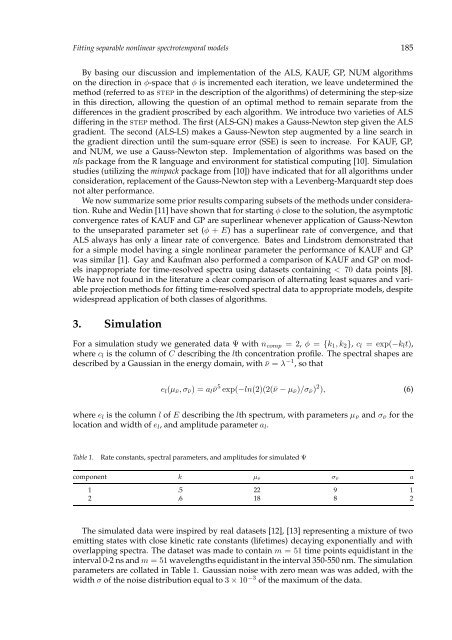
Fitting separable nonlinear spectrotemporal models 185By basing our discussion and implementation of the ALS, KAUF, GP, NUM algorithmson the direction in φ-space that φ is incremented each iteration, we leave undetermined themethod (referred to as step in the description of the algorithms) of determining the step-sizein this direction, allowing the question of an optimal method to remain separate from thedifferences in the gradient proscribed by each algorithm. We introduce two varieties of ALSdiffering in the step method. The first (ALS-GN) makes a Gauss-Newton step given the ALSgradient. The second (ALS-LS) makes a Gauss-Newton step augmented by a line search inthe gradient direction until the sum-square error (SSE) is seen to increase. For KAUF, GP,and NUM, we use a Gauss-Newton step. Implementation of algorithms was based on thenls package from the R language and environment for statistical computing [10]. Simulationstudies (utilizing the minpack package from [10]) have indicated that for all algorithms underconsideration, replacement of the Gauss-Newton step with a Levenberg-Marquardt step doesnot alter performance.We now summarize some prior results comparing subsets of the methods under consideration.Ruhe and Wedin [11] have shown that for starting φ close to the solution, the asymptoticconvergence rates of KAUF and GP are superlinear whenever application of Gauss-Newtonto the unseparated parameter set (φ + E) has a superlinear rate of convergence, and thatALS always has only a linear rate of convergence. Bates and Lindstrom demonstrated thatfor a simple model having a single nonlinear parameter the performance of KAUF and GPwas similar [1]. Gay and Kaufman also performed a comparison of KAUF and GP on modelsinappropriate for time-resolved spectra using datasets containing < 70 data points [8].We have not found in the literature a clear comparison of alternating least squares and variableprojection methods for fitting time-resolved spectral data to appropriate models, despitewidespread application of both classes of algorithms.3. SimulationFor a simulation study we generated data Ψ with n comp = 2, φ = {k 1 , k 2 }, c l = exp(−k l t),where c l is the column of C describing the lth concentration profile. The spectral shapes aredescribed by a Gaussian in the energy domain, with ¯ν = λ −1 , so thate l (µ¯ν , σ¯ν ) = a l¯ν 5 exp(−ln(2)(2(¯ν − µ¯ν )/σ¯ν ) 2 ), (6)where e l is the column l of E describing the lth spectrum, with parameters µ ¯ν and σ¯ν for thelocation and width of e l , and amplitude parameter a l .Table 1.Rate constants, spectral parameters, and amplitudes for simulated Ψcomponent k µ¯ν σ¯ν a1 .5 22 9 12 .6 18 8 2The simulated data were inspired by real datasets [12], [13] representing a mixture of twoemitting states with close kinetic rate constants (lifetimes) decaying exponentially and withoverlapping spectra. The dataset was made to contain m = 51 time points equidistant in theinterval 0-2 ns and m = 51 wavelengths equidistant in the interval 350-550 nm. The simulationparameters are collated in Table 1. Gaussian noise with zero mean was was added, with thewidth σ of the noise distribution equal to 3 × 10 −3 of the maximum of the data.