SECTION 1 - Boat Design Net

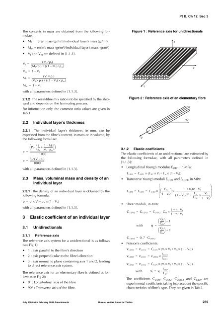
Pt B, Ch 12, Sec 3The contents in mass are obtained from the following formulae:• M f = fibres’ mass (gr/m 2 )/individual layer’s mass (gr/m 2 )• M m = resin’s mass (gr/m 2 )/individual layer’s mass (gr/m 2 )• V f and V m are defined in [1.1.3].V f =( M f ⁄ ρ f )-------------------------------------------------------------( M f ⁄ ρ f ) + (( 1 – M f ) ⁄ ρ m )V m = 1 – V fM f =( V f × ρ f )---------------------------------------------------------------( V f × ρ f ) + (( 1 – V f ) × ρ m )M m = 1 – M fwith all parameters defined in [1.1.3].2.1.2 The resin/fibre mix ratio is to be specified by the shipyardand depends on the laminating process.For information only, the common ratio values are given inTab 1.2.2 Individual layer’s thickness2.2.1 The individual layer’s thickness, in mm, can beexpressed from the fibre’s content, in mass or in volume, bythe following formulae:⎛ 1 1 – MP f ⋅ ⎛---+ ---------------- f ⎞⎞⎝ ⎝ρ f M f ⋅ ρ m⎠⎠e = ------------------------------------------------1000Pe f ⁄ ( V f ⋅ ρ f )= --------------------------1000with all parameters defined in [1.1.3].2.3 Mass, voluminal mass and density of anindividual layer2.3.1 The density of an individual layer is obtained by thefollowing formula:ρ = ρ f × V f + ρ m × ( 1 – V f )with all parameters defined in [1.1.3].3 Elastic coefficient of an individual layer3.1 Unidirectionals3.1.1 Reference axisThe reference axis system for a unidirectional is as follows(see Fig 1):• 1 : axis parallel to the fibre’s direction• 2 : axis perpendicular to the fibre’s direction• 3 : axis normal to plane containing axis 1 and 2, leadingto direct reference axis system.The reference axis for an elementary fibre is defined as follows(see Fig 2):• 0° : Longitudinal axis of the fibre• 90° : Transverse axis of the fibre.Figure 1 : Reference axis for unidirectionalsFigure 2 : Reference axis of an elementary fibre0°3.1.2 Elastic coefficientsThe elastic coefficients of an unidirectional are estimated bythe following formulae, with all parameters defined in[1.1.3]:• Longitudinal Young’s modulus E UD1 , in MPa:E UD1 = C UD1 × ( E f0° × V f + E m × ( 1 – V f ))• Transverse Young’s moduli E UD2 and E UD3 , in MPa:⎛⎞2⎜ EE UD2 E UD3 C ⎛ mUD2-------------- ⎞ 1 + 0,85 ⋅ V f⎟= = × ⎜ × ----------------------------------------------------------------⎝ 21 – ν ⎠⎟⎜ m( 1 – V f ) 1,25 E--------- m V+ × -------------- f ⎟⎝2E f90° 1 – ν ⎠m• Shear moduli, in MPa:1 + η ⋅ VG UD12 = G UD13 = C UD12 ⋅ G × ---------------------- fm1 – η ⋅ V fwith⎛-------⎞ – 1⎝G m⎠η = ----------------------⎛ G------- f ⎞ + 1⎝ ⎠G UD23 = 0, 7 ⋅ G UD12• Poisson’s coefficients:ν UD13 = ν UD12 = C UDν × ( ν f × V f + ν m × ( 1 – V f ))G fG mEν UD21 = ν UD31 = ν UD2UD12 × ----------E UD1The coefficients C UD1 , C UD2 , C UD12 and C UDν areexperimental coefficients taking into account the specificcharacteristics of fibre’s type. They are given in Tab 2.!90°′ν UD23 = ν UD32 = C UDν × ( ν f × V f + ν m × ( 1 – V f ))′ Ewith ν f = νf90°f ⋅ ---------E f0°July 2006 with February 2008 Amendments Bureau Veritas Rules for Yachts 289