Theoretical and Experimental DNA Computation (Natural ...

4.8 Example Application: Transitive Closure 89
we concentrate on the all-pairs transitive closure problem. Here, we find all
pairs of vertices in the input graph that are connected by a path.
The transitive closure of a directed graph G =(V,E) is the graph G ∗ =
(V,E ∗ ), where E ∗ consists of all pairs , such that either i = j or there
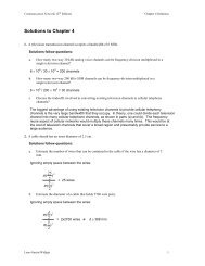
exists a path from i to j. An example graph G is depicted in Fig. 4.7a with
its transitive closure G ∗ depicted in Fig. 4.7b.
1 2
5
3 4
(a)
1 2
5
3 4
(b)
Fig. 4.7. (a) Example graph, G. (b) Transitive closure of G
We represent G by its adjacency matrix, A. LetA ∗ be the adjacency matrix
of G ∗ .In[83],JàJà shows how the computation of A ∗ may be reduced to
computing a power of a Boolean matrix.
We now describe the structure of a NAND gate Boolean circuit to compute
the transitive closure of the n×n Boolean matrix A. For ease of exposition
we assume that n =2 p .
The transitive closure, A ∗ ,ofA is equal to (A + I) n ,whereI is the n × n
identity matrix. This is computed by p =log 2 n levels. The i th level takes
as input the matrix output by level i − 1 (with level 1 accepting the input
matrix A + I) and squares it: thus level i outputs a matrix equal to (A + I) 2i
(Fig. 4.8).
To compute A 2 given A, then 2 Boolean values A 2 i,j
(1 ≤ i, j ≤ n) are
needed. These are given by the expression A2 i,j =
n
∨
k=1Ai,k ∧ Ak,j. First, all the
n3 terms Ai,k ∧ Ak,j (for each 1 ≤ i, j, k ≤ n) are computed in two (parallel)
steps using two NAND gates for each ∧-gate simulation. Using NAND gates,
we have x ∧ y = NAND(NAND(x, y),NAND(x, y)). The final stage is to
n
∨
k=1 (Ai,k ∧ Ak,j) that form the input to the
compute all of the n2 n-bit sums
next level.
n
∨
The n-bit sum k=1 xk, can be computed by a NAND circuit comprising
p levels each of depth 2. Let level 0 be the inputs x1,...,xn; level i has 2p−i outputs y1,...,yr, andleveli + 1 computes y1 ∨ y2,y3 ∨ y4,...,yr−1 ∨ yr.